
Translation note. This is a faithful translation of the Swedish master. Equations, numerical values, source-code listings, reconstruction notes, and Pass 2 checkpoints have been preserved without technical correction.
MASTER’S THESIS IN ELECTRICAL POWER CONVERSION
Study of harmonic losses in an induction machine connected in series with an inductor. 🇬🇧
Supervisor: Tom Porteous
Submitted: 1979-11-27
Status: Approved
Abstract
This master’s thesis was carried out at the High-Power Laboratory of ASEA’s Central Development Department in Västerås. The supervisor was Tom Porteous.
The purpose of the work was to study the effect of a series inductor on the operating conditions of an inverter-fed induction machine, with respect to derating and torque pulsations, and, if possible, to identify an optimal combination of motor and inductor.
The calculations were performed using computer programs applied to an ASEA standard motor, MBK 280 S-6, rated at 75 kW. Data from laboratory tests concerning iron losses were added to these calculations. The results were then used to assess the loss reductions obtainable with different inductor sizes. The physical dimensions of the inductor were also taken into account in this assessment.
The thesis shows that when motor space is limited, there is no reason, from a loss perspective, to introduce a series inductor into the system, because the combined weight of motor and inductor is essentially constant.
When motor space is unrestricted, however, the results show that a series inductor can be used advantageously up to a limiting frequency specific to each inductor, in order to reduce torque derating. Once this limiting frequency is exceeded, the inductor should be disconnected. This minimizes derating at high frequencies, but increases torque pulsations.
Table of Contents
1. $~$ Introduction
$\quad$ 1.1 $~$ General
$\quad$ 1.2 $~$ Supply
$\quad$ 1.3 $~$ Disadvantages of PWM Supply
$\quad$ 1.4 $~$ Measures
$\quad$ 1.5 $~$ Methods
2. $~$ Iron Losses
$\quad$ 2.1 $~$ General
$\quad$ 2.2 $~$ Difficulties in the Analytical Determination of Iron Losses
$\quad$ 2.3 $~$ Method
$\quad$ 2.4 $~$ No-Load Operation without a Series Inductor
$\quad$ 2.5 $~$ No-Load Operation with a Series Inductor
$\quad$ 2.6 $~$ Analysis
3. $~$ The Motor under Load
$\quad$ 3.1 $~$ General
$\quad$ 3.2 $~$ Load without a Series Inductor
$\quad$ 3.3 $~$ Dependence of Losses on Inductance
$\quad$ 3.4 $~$ Dependence of Losses on Frequency
$\quad$ 3.5 $~$ Torque Pulsations
$\quad$ 3.6 $~$ Weight Calculation
4. $~$ Discussion
$\quad$ 4.1 $~$ Capabilities and Limitations of the Procedure
$\quad$ 4.2 $~$ Inductor Size with Unrestricted Motor Space
$\quad$ 4.3 $~$ Inductor Size with Limited Motor Space
5. $~$ References
Appendices
B1: $~$ Diagrams
B2. $~$ Supply-Voltage Waveform and Fourier Analysis
B3. $~$ Calculation Model
B4: $~$ Program Description: PWMIND
B5. $~$ Calculation of Inductor Size
B6: $~$ Type Data
B7. $~$ List of Variables
1. Introduction
1.1 General
In recent years, a new type of motor drive has emerged and attracted considerable interest among motor manufacturers. In traction applications, among others, inverter-fed induction machines have begun to compete seriously with thyristor-rectifier-fed DC motors. The advantages are numerous: for example, the induction motor is considerably more robust than the DC motor, requires substantially less maintenance, and performs better in harsh environments. Standard motors can also often be used, reducing prices and simplifying service. As the prices of thyristors and their auxiliary electronics have fallen, the inverter-and-induction-motor alternative has therefore become increasingly competitive.
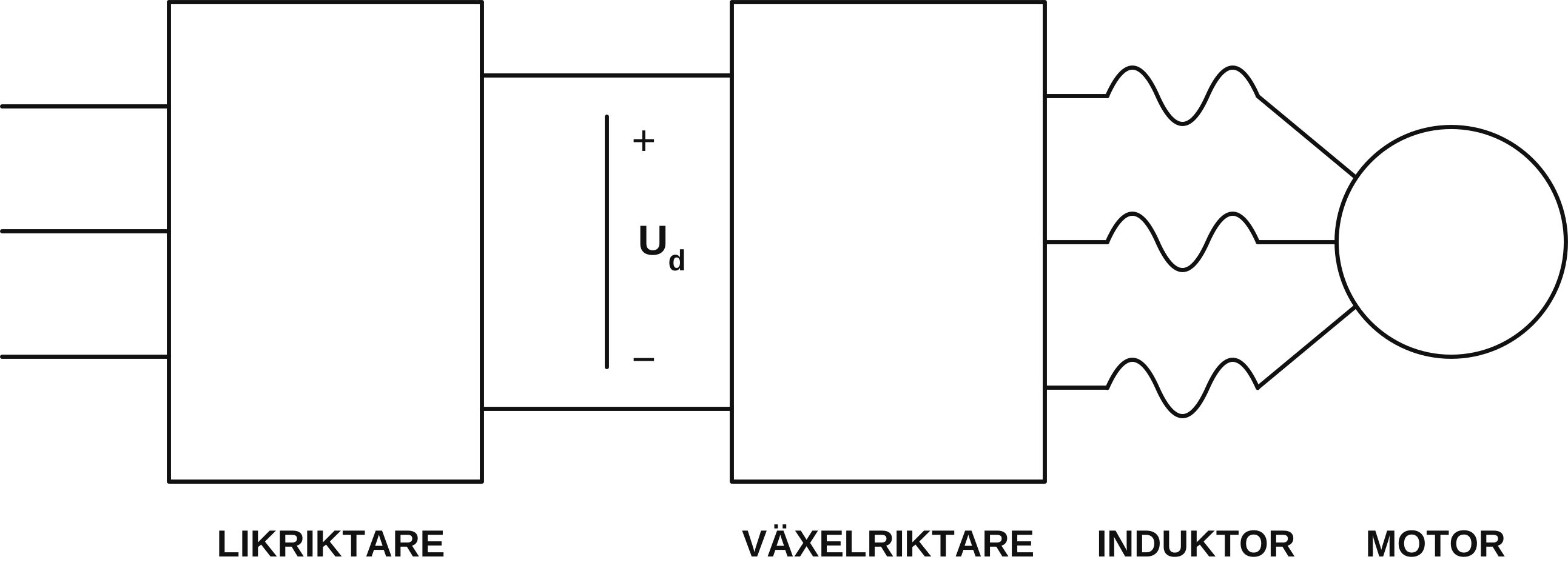
1.2 Supply
An induction motor can be supplied at variable frequency using either voltage-source or current-source converters. In this case, a voltage-source inverter has been used.
It rectifies the AC voltage from the supply network into a constant DC-link voltage $U_d$ (Figure 1). An AC voltage is then obtained by chopping the DC-link voltage in the thyristor bridge and multiplying it by a modulation voltage to obtain variable frequency and amplitude (see Appendix 2).
At low frequencies, the chopping is performed in such a way that the harmonic distribution is altered and the fifth and seventh harmonics are suppressed, which provides certain operating advantages (see Section 3). The reference and modulation voltages may therefore have the form shown in Figure 2.
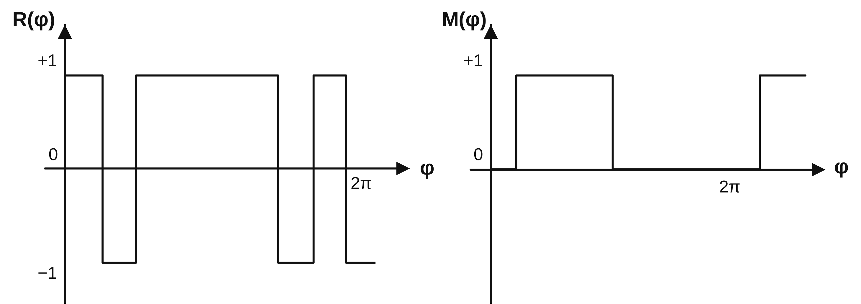
This produces an AC voltage of arbitrary frequency and amplitude. The maximum fundamental amplitude is obtained when the modulation voltage is constant—that is, when the entire reference signal is passed through—and is limited by the DC-link voltage.
This type of supply is called PWM supply (pulse-width modulation), because the magnitude of the fundamental voltage is determined by the width of the modulation pulses, not by the amplitude of the reference signal.
As the inverter frequency is varied from 0 to 50 Hz, it passes through a number of operating modes (see Appendix 6). At predetermined frequencies, the supply-voltage waveform is changed so that an optimal supply can be maintained. Notches are introduced into the reference voltage to suppress low-order harmonics at low frequencies, and the frequency of the modulation voltage is changed so that it is a multiple of six times the frequency of the reference signal.
1.3 Disadvantages of PWM Supply
The inverter stage delivers an essentially square-wave voltage to the motor. This generates harmonics, which in turn create additional losses in the rotor and stator (iron and copper) without contributing additional torque. As a result, the motor must be derated relative to operation with a conventional sinusoidal supply.
Another problem is that the high harmonic content produces undesirable torque pulsations about the load torque, which can be substantial, particularly at low frequencies. In traction applications, for example, the torque pulsations can cause wheel slip during starting.
They can also create negative torque that is transmitted through the motor to mechanical couplings in the system. The resulting mechanical stresses are large and are regarded as very serious.
For this reason, the supply voltage is notched so that the fifth and seventh harmonics are suppressed and the largest pulsations disappear. It should be noted, however, that this merely redistributes the harmonics: the amplitudes of higher-order harmonics increase when the fifth- and seventh-harmonic voltages decrease. A further problem is that the supply-voltage waveform makes the motor extremely noisy.
1.4 Measures
In addition to the redistribution of harmonics described above, one method of reducing the harmonic content in the motor is to filter the supply voltage. A series inductor is therefore inserted in each of the three phases between the inverter and the motor, reducing the harmonic amplitudes relative to the fundamental. This is the subject studied in the present report.
1.5 Methods
To determine the magnitude of the losses and pulsations, Fourier analysis of the supply voltage has been applied (see Appendix 2). When applied to the conventional machine model (Figure 3), and with account taken of the current-displacement phenomenon in the rotor, this gives the contribution of each harmonic to the copper losses and the total torque pulsation about the load torque.
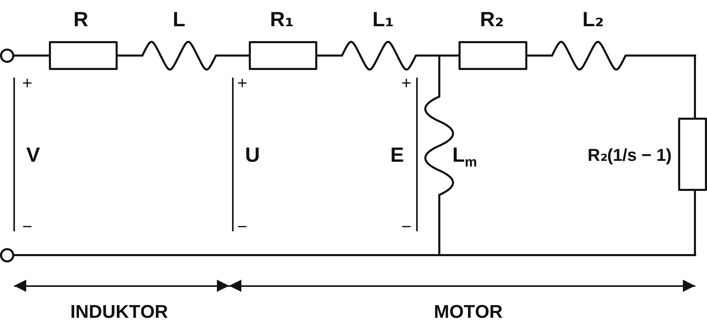
These theories are incorporated in the computer program PWMIND (pulse-width modulation with an inductor; see Appendix B.4). Estimated iron losses were added to the results obtained from the program.
All of this, applied to an ASEA standard motor (MBK 280 S-6, no. 7125 824) with forced cooling and used together with a series inductor, formed the basis for evaluating which inductor could, for electrical, mechanical, and physical reasons, be regarded as the best—if not strictly optimal—solution to the problem. These conclusions are drawn for the standard motor in question, but can also be applied to other combinations of motor and inductor.
2. Iron Losses
2.1 General
The motor derating is obtained by determining the total losses in the motor. Hereafter, total losses means the sum of copper and iron losses; friction and stray-load losses are not included. The iron losses are therefore first determined from no-load tests. They are then added to the copper losses obtained under load, and the derating is calculated (see The Motor under Load).
2.2 Difficulties in the Analytical Determination of Iron Losses
Calculating the iron losses analytically can be difficult. The losses are divided into two components: hysteresis losses and eddy-current losses. Thus:
\[P_{fe} = P_v + P_h\] \[P_h = k_h f B_{\max}^{\lambda} \qquad 1 < \lambda < 3\] \[P_v = k_v \sigma d^2 f^2 B^2\](List of variables in Appendix 7.)
Because the relationship between $P_v$ and $P_h$ is unknown, the frequency and voltage dependence of the variables involved is not known, and superposition cannot be applied, iron-loss calculations clearly present certain difficulties.
2.3 Method
An alternative method is to measure the no-load losses occurring at different frequencies and subtract from them the copper-loss values calculated from the machine model when the machine is operating at no load with respect to the fundamental (the harmonics simultaneously operate at a slip of one). The remaining losses are then postulated to be iron losses. This method at least provides an absolute upper bound for the magnitude of the iron losses.
2.4 No-Load Operation without a Series Inductor
The total losses (iron + copper) were measured on an ASEA standard motor, MBK 280 S-6, with forced cooling under both PWM and sinusoidal supply. The copper losses calculated with the PWMIND computer program were then subtracted from the total losses, yielding the remaining iron losses. Appendix 1.1 plots both the total no-load losses under PWM supply and the calculated iron losses under PWM and sinusoidal supply as functions of frequency. The dashed line for the PWM iron losses should be regarded as a trend. In these measurements and calculations, the fundamental flux was the same under PWM and sinusoidal operation.
The abrupt jumps in the total and PWM iron losses are caused by the operating-mode changes introduced at ten frequencies (see the Introduction and Appendix 6) to reduce the losses. The fact that the no-load copper losses amount to almost fifty percent of the total losses under PWM supply is due to the additional losses produced by the harmonics. Consequently, no-load losses cannot be treated as iron losses.
The harmonics also explain why losses at low frequencies within an operating mode can be greater than at a higher frequency: the relative harmonic content (the ratio of harmonic amplitude to fundamental amplitude) is greater.
To provide a basis for comparison, the sinusoidal-supply iron losses were determined in the corresponding manner (total loss minus copper loss). Comparison shows that the PWM iron losses are considerably greater than the sinusoidal losses, again because of the harmonics. In this case, the conclusion is that the PWM iron losses exceed those under sinusoidal supply by an approximately constant term of about 1 kW. Consequently, particularly at lower frequencies, the relative increase in iron losses is very large.
2.5 No-Load Operation with an Inductor
After studying the relationships between the no-load losses under PWM and sinusoidal supply, a series inductor is introduced into the circuit (as shown in Figure 3). Because the motor impedance is dominated by reactance, the inductor will not act as a first-order low-pass filter, but rather as an element in a voltage divider. It attenuates the harmonic amplitudes and thereby substantially improves the voltage waveform at the motor terminals ($U$). This improved waveform reduces harmonic losses (both copper and iron), as reflected in Appendices 1.1–1.3, all three of which show total and iron losses at no load as functions of frequency for different inductances.
The proportion of copper losses in the total no-load losses decreases substantially as inductor size increases, but is still as high as one-half of the total loss at 0.21 pu (1 mH) and 10 Hz. (The per-unit values are referenced to the motor’s rated voltage and rated current; the base impedance then corresponds to $Z_B$ = 1.47 mH and the base inductance is $L_B$ = 4.67 mH according to Appendix 6; the short-circuit reactance is approximately 0.25 pu.) The fundamental-voltage drop across the inductor has been taken into account here, and a correction term has been introduced between the different curves so that all three curves are fully comparable (this also applies to the sinusoidal-supply curve).
2.6 Analysis
It is therefore difficult to determine the iron losses analytically, but the problem can be restricted to deriving the curves with an inductor (Appendices 1.2–1.3) from the curve without a series inductor (Appendix 1.1). Examination of the equivalent circuit for the different harmonics shows that, at no load, the slip is approximately zero for the fundamental.
This makes the rotor resistance very large, and the only fundamental current that flows is the magnetizing current. If the stator resistance is neglected, the fundamental current on the stator side is:
\[I_{11} = \frac{V_1-E_1}{X_1+X}\] \[E_1 = X_m I_{11}\] \[I_{11} = \frac{V_1}{X_1+X_m+X}\]In contrast, the slip is considerably greater for the harmonics ($s \approx 1$). The rotor resistance is then low, and the magnetizing reactance is largely shunted by the rotor impedance. The harmonic currents on the stator side equal those on the rotor side and, if the resistances are neglected:
\[I_{1\ddot{o}} = I_{2\ddot{o}} = \frac{V_{\ddot{o}}}{X_1+X_2+X}\]Comparison of the cases with and without a series inductor therefore shows that the fundamental current is reduced by the factor
\[\frac{X_1+X_m}{X_1+X_m+X}\]whereas the harmonic current is reduced by the factor
\[\frac{X_1+X_2}{X_1+X_2+X}.\]Because $X_m$ is considerably greater than $X$, $X_1$, and $X_2$, the reduction in the fundamental is moderate. Consequently, the fundamentals of the inverter-terminal voltage and motor-terminal voltage are approximately equal ($V_1 \approx U_1$). For the harmonics, $X$, $X_1$, and $X_2$ are comparable. Voltage division therefore gives
\[U_ö \approx V_ö \frac{X_1+X_2}{X_1+X_2+X}.\]If the harmonic iron losses can be assumed proportional to the square of the harmonic voltages, the following should apply:
\[P_{feö}(X) = P_{feö}(X=0) \frac{(X_1+X_2)^2}{(X_1+X_2+X)^2}.\]If the difference between the total iron loss and the fundamental iron loss (the sinusoidal loss) is reduced by this factor and plotted above the fundamental iron loss, the dotted values in Appendices 1.2–1.3 are obtained. As shown, these agree well with the values calculated from the total no-load losses (crosses). (These arguments are unaffected by current displacement, because it is equally large for each corresponding harmonic in the three cases.)
3. The Motor under Load
3.1 General
So far, the losses have been studied only at no load. To reach the practically relevant case, the motor is now loaded. The slip then increases, and greater current and power are drawn. Copper losses rise, and under PWM supply the total losses (copper and iron) can amount to approximately 10 kW for a motor rated at 75 kW.
Losses in excess of those at rated load under sinusoidal supply result in motor derating. Derating means that less torque must be drawn from the motor to keep the loss power down, and larger motors are therefore required for a given load torque. If a series inductor is inserted in the circuit, the additional losses can be reduced and the derating factor improved.
Under load, the voltage drop across the inductor is no longer negligible (because the increased slip shunts the magnetizing reactance even for the fundamental). A trade-off must therefore be made between the inductor’s negative voltage-reducing effect and its positive attenuation of harmonic losses in the motor. Balancing these effects might appear to yield a minimum loss, were it not for the fact that losses decrease with the square of voltage while motor voltage decreases linearly. The largest possible inductance is therefore appropriate when voltage and space are unrestricted, in order to reduce derating in a given motor.
3.2 Load without a Series Inductor
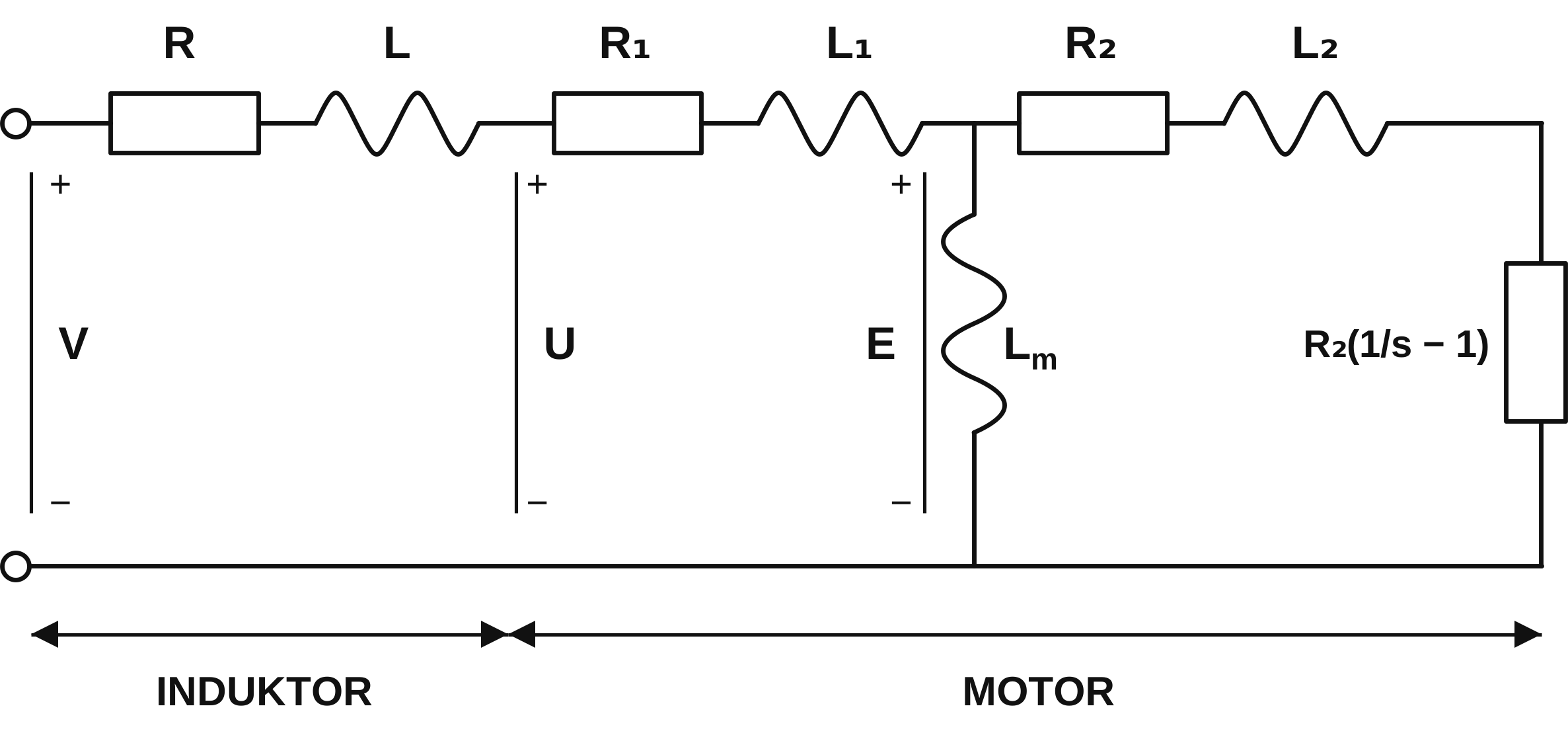
The general conditions are first studied when the motor is not supplied through a series inductor. The computer program was used to calculate the copper losses for two different cases: first, when the fundamental ($V_1$) of the supply voltage ($V$)—here equal to $U$—was made directly proportional to frequency; and second, when the flux was held constant. The latter means that the voltage $E_1$ (see Figure 4) must vary linearly with frequency because
\[E_1 \sim j\omega\Psi_1 \sim j\omega\Phi_1\]The first case does not produce constant flux because, at low frequencies, the resistances become comparable to the reactances, and $E_1$ is then no longer a simple, non-phase-shifted linear function of $V_1$.
The effect of this can be seen in Appendix 1.4, Figure 1. The figure shows the total motor losses at constant torque (700 Nm) as a function of frequency. Curve A represents the first case, in which the fundamental of the inverter-terminal voltage is $V_1 = kf$. The sinusoidal case was calculated correspondingly, producing curve a. In case A, the derating (Appendix 1.4, Figure 2), $\xi = 1 - M/M_n$, becomes very large. Since $M\propto I$ and $P_{cu}\propto I^2$, it follows that $\xi = 1- \sqrt{P_{cun} / {P_{cu}}}$. On this basis, the derating is greatest at low frequencies under PWM supply ($\xi$ = 18% at 11 Hz). These calculations assume that forced cooling can remove all losses effectively, regardless of speed. In practice, this has proved difficult to achieve, so an additional correction term must be introduced to account for this effect.
When the flux is held constant, the conditions are different. The sinusoidal losses then decrease at low frequencies because the copper losses are constant ($\Phi=\text{constant} \Rightarrow I=\text{constant}$) and the iron losses decrease with frequency (curve b). In the PWM case, a loss maximum occurs at approximately 30 Hz (curve B), and the derating is approximately 14%.
It can therefore be noted that, under PWM operation at constant flux, the derating can vary between approximately 8% and 14%, and that the losses are greatest at 30 Hz.
3.3 Dependence of Losses on Inductance
Appendix 1.5 was prepared to study how the inductor affects the losses at a given frequency. The load torque was 700 Nm and the frequency 30 Hz. The figure shows both the copper losses under load—divided into fundamental loss ($P_{cu1}$) and harmonic losses ($P_{cuö}$)—and the supply voltage $V_1$ as a function of frequency.
As with the iron losses, one can write
\[P_{cuö}(X) = P_{cuö}(X=0) \frac{(X_1+X_2)^2}{(X_1+X_2+X)^2}.\]The order of magnitude of the inductor is therefore in the vicinity of the short-circuit reactance
\[X_k=X_1+X_2,\]that is, approximately 0.25 pu (see Appendix 6). The diagram in Appendix 1.5 shows the values calculated by the program (crosses) and the values obtained from the expression above and combined with the fundamental loss (dots). Once again, the agreement is good. The quadratic decrease means that the harmonic losses have been reduced by a factor of four when
\[X=X_1+X_2=X_k,\]which may be regarded as a rough rule of thumb for the required inductor size. It is also worth noting how rapidly the required supply voltage rises with inductance. If the inductance is slightly greater than 4 mH (0.86 pu), a supply voltage $V$ of 220 $V_{eff}$ is required, corresponding to maximum utilization of the 488 V DC-link voltage. At still larger inductances, constant flux cannot be maintained.
3.4 Dependence of Losses on Frequency
The effect of the inductor on the losses can also be calculated as a function of frequency. For a given inductance and load torque, the minimum copper losses are obtained if the motor flux is held constant, irrespective of frequency.
This in turn requires the supply voltage to be increased to compensate for the voltage drop across the inductor and stator. At low frequencies this is possible because the full available voltage (here $V_1$ = 220 V) is not yet being used. As the frequency rises, however, a frequency specific to each inductor is reached at which no more voltage can be obtained from the DC link. Beyond this limit, the constant-flux requirement must be abandoned in favor of the constant-torque requirement, which is met by increasing the slip.
The effect can be studied in Appendices 1.6 and 1.7. If there is no inductor in the circuit, the problem does not arise and the curve has the form shown for $L$ = 0. The other curves would have the same convex form were it not for the voltage ceiling described above. For the 1 mH (0.22 pu) curve, for example, this becomes apparent at approximately 44 Hz. Above this frequency, the losses rise sharply because of the increased current (up to this frequency, constant flux has produced essentially constant current, $s \propto 1/\textit{f}$). The effect is even more pronounced in the 2 mH (0.43 pu) case. The voltage drop across the inductor then becomes so large that 700 Nm cannot be obtained at high frequencies. It therefore appears appropriate to bypass the inductor at a limiting frequency determined by the point at which total losses with and without the inductor are equal. At frequencies above the specific limiting frequency, the losses then follow the curve for $L$ = 0.
If this is done and the required derating is calculated from the losses, Appendix 1.7 is obtained. It shows that a large inductance reduces derating at low frequencies, but produces a large variation in derating. A small inductor instead gives a more uniform derating curve.
3.5 Torque Pulsations
The harmonic content of the supply voltage produces torque pulsations about the mean torque, and these must be taken into account. They become particularly significant at low frequencies, which is why the method of suppressing the fifth and seventh harmonics (see Appendix 2) is used to redistribute the harmonics. Appendix 1.8, Figure 1, and Appendix 1.9 show the maximum and minimum values of total torque at 700 Nm and 0 Nm ($\propto M_n$ and $\Theta$) as functions of frequency. The torque values were obtained from the computer program, which also accounts for the elimination of low-order harmonics. The curves provide only an overview of the pulsations about the mean torque and their frequency dependence. If plotted with more points, the jumps at the operating-mode transitions would be more apparent.
Disconnecting, for example, a 1 mH (0.22 pu) inductance at 47 Hz would increase the pulsations from approximately ±150 Nm to ±300 Nm, which is not particularly significant when the torque is 700 Nm. At low load, however, it represents a doubling.
The curves in Appendix 1.8, Figure 1, and Appendix 1.9 also show that the pulsations are approximately constant and independent of load torque.
The reduction in pulsation as a function of inductance can be seen in Appendix 1.8, Figure 2. The pulsating torque is proportional to current and should therefore, in accordance with the preceding calculations, be given by
\[M_p(X) = M_p(X=0) \frac{X_1+X_2}{X_1+X_2+X}.\]This corresponds to the dots, which agree well with the crosses obtained from the program.
3.6 Weight Calculation
A weight calculation may be useful in determining whether a minimum combined motor-and-inductor weight can be found at rated torque. The weight is calculated as follows:
For each specified inductance, a motor weight and an inductor weight are calculated. The motor weight is obtained from data for the MBK 280 S-6S. Weight as a function of the length of the active rotor and stator parts is determined from the data in Appendix 6. The length of the active parts is then assumed to be directly proportional to the loss power. Inductor weight as a function of inductance is obtained from Appendix 5, in which an air-cooled inductor has been optimized.
The weights are plotted in Appendix 1.10. It shows that the minimum in the weight curve is very shallow: the saving in motor size is offset by the weight of the inductor. This does not, however, account for the benefits in torque pulsation or for the amount of space available.
4. Discussion
4.1 Capabilities and Limitations of the Procedure
The calculation procedure developed here makes it possible, for an arbitrary motor–inductor combination, to determine the distribution and magnitude of losses, voltage drops, and derating at different frequencies and voltages. Together with information on the physical dimensions of the motor and inductor and the available space, this provides a basis for selecting the motor–inductor combination.
The accuracy of the procedure is limited to some extent by the assumption of a square-wave voltage with vertical edges. In reality, the harmonic content is therefore lower and the losses are somewhat smaller. This reduction is partly offset by the fact that friction losses have not been included.
One limitation of the calculation routine is that the corresponding iron losses under PWM supply cannot be calculated from a given iron loss under sinusoidal supply. On the basis of Appendix 1.1, however, the general conclusion can be drawn that the iron losses under PWM supply exceed those in the sinusoidal case by an approximately constant term across different frequencies, and that the PWM iron losses at 50 Hz are approximately twice the sinusoidal iron losses at the same frequency.
This entire study is based on the assumption that forced cooling provides effective cooling at all frequencies. In practice, however, this is not the case, and the derating will increase further by a factor that depends on the cooling conditions in each specific application.
4.2 Inductor Size with Unrestricted Motor Space
If the motor is to be used in an environment where the space available for the motor and inductor is essentially unrestricted, Appendix 1.10 shows that using a series inductor produces no appreciable saving. From this perspective, there is therefore no reason to use the series inductor, except to limit torque pulsations.
4.3 Inductor Size with Limited Motor Space
If the dimensions of the motor space are fixed, as in the bogie of a locomotive, for example, the weight argument no longer applies. The objective is then to obtain the maximum torque from a given motor. In such cases, the inductor should be selected large enough to provide a reasonable reduction in harmonics. The harmonic losses as a function of inductance can be expressed approximately as:
\[P_{cuö}(X) = P_{cuö}(X=0) \frac{(X_1+X_2)^2}{(X_1+X_2+X)^2},\] \[P_{feö}(X) = P_{feö}(X=0) \frac{(X_1+X_2)^2}{(X_1+X_2+X)^2},\] \[X_1+X_2 \approx X_k.\]Reducing the harmonic losses to one-quarter of the losses without an inductor therefore requires an inductor $L=L_k$. This also halves the torque pulsations
\[M_p(X) = M_p(X=0) \frac{X_1+X_2}{X_1+X_2+X}.\]The inductor should be selected in this order of magnitude. A smaller inductor produces no appreciable improvement compared with operation without an inductor, whereas a large inductor—for example, $L=2 \times L_k$—provides only very small marginal improvements.
A large inductor also has a low limiting frequency at which the flux can no longer be held constant in the motor and the motor losses increase (Appendices 1.6 and 1.7). Regardless of inductor size, the inductor should be disconnected at the frequency at which the losses with and without the inductor in the circuit are equal.
5. References
P. Krause, Method of multiple reference frames applied to the analysis of symmetrical induction machinery. IEEE Transactions on Power Apparatus and Systems, vol. PAS-87, no. 1, pp. 218-226.
F. G. G. de Buck, Design adaption of inverter supplied induction motors. Electric Power Applications, May 1978, vol. 1, no. 2, pp. 54-60.
E. Alm, Electrical Engineering, Volume III: Electrical Machinery, Part 2A, 1927, pp. 356–362.
F. Gustavson, Compendium in Electromechanical Energy Conversion, Part 1, 1978, pp. 4.1–4.20.
T. Porteous, Program Descriptions for PWMOT and RESIST.
Appendices
Appendix B1 consists primarily of diagrams and has been omitted. They are available in the original photostat copy.
Appendix B2. Supply-Voltage Waveform and Fourier Analysis
B2.1 Waveform
In the simplest case, the inverter can supply a square-wave voltage (the reference voltage) multiplied by a modulation voltage consisting of pulses whose widths are modulated. Such a supply, however, produces severe fifth- and seventh-harmonic pulsations, especially at low frequencies. To eliminate these, the reference voltage is notched so that these low-order harmonics are shifted to higher frequencies.
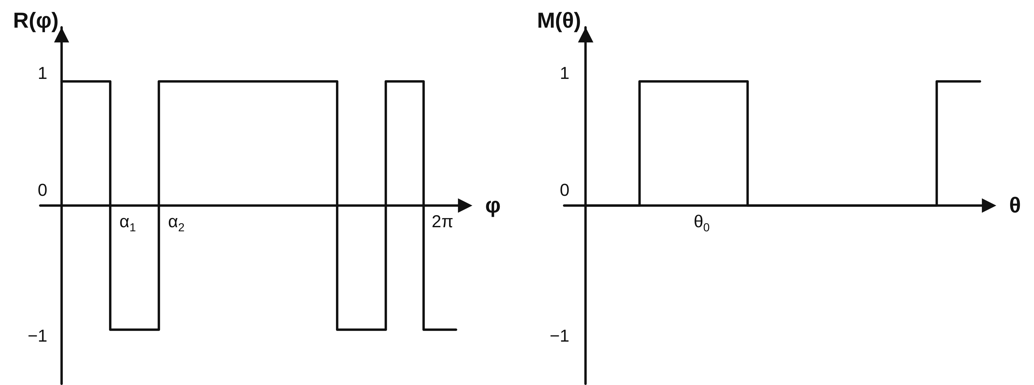
These two signals are expanded in Fourier series and multiplied by one another.
B2.2 Fourier Expansion
$R(\varphi)$ is an odd function. Its Fourier expansion therefore contains only sine terms.
The number of notches may be assumed even, because an odd number of notches can be converted into an even number without changing the conditions (place one notch at $\pi/2$).
\[\begin{aligned} R_n &= \frac{1}{\pi}\int_0^{2\pi} R(\varphi)\sin(n\varphi)\,d\varphi \\ &= \frac{4}{\pi}\int_0^{\pi/2} R(\varphi)\sin(n\varphi)\,d\varphi \\ &= \frac{4}{\pi}\left[ \int_0^{\pi/2}\sin(n\varphi)\,d\varphi -2\sum_{k=1}^{j} \int_{\alpha_{2k-1}}^{\alpha_{2k}}\sin(n\varphi)\,d\varphi \right] \\ &= \{\text{the unnotched signal minus the notches}\} \\ &= \frac{4}{n\pi}\left[ 1+2\sum_{k=1}^{j} \left(\cos(n\alpha_{2k})-\cos(n\alpha_{2k-1})\right) \right]. \end{aligned}\]That is,
\[R_n = \frac{4}{n\pi} \left[ 1+2\sum_{k=1}^{2j}(-1)^k\cos(n\alpha_k) \right].\]$M(\theta)$ is an even function. Its Fourier expansion therefore contains only cosine terms.
\[\begin{aligned} M_i &= \frac{1}{\pi}\int_{-\pi}^{\pi}M(\theta)\cos(i\theta)\,d\theta \\ &= \frac{2}{\pi}\int_0^{\pi}M(\theta)\cos(i\theta)\,d\theta \\ &= \frac{2}{\pi}\int_0^{m\pi}\cos(i\theta)\,d\theta \\ &= \frac{2}{i\pi}\sin(i m\pi). \end{aligned}\] \[M_0=\text{mean value of the modulation signal}=m.\]This gives the Fourier series of $M$, including the phase shift:
\[M(\theta-\theta_0) = m+\sum_{i=1}^{\infty}M_i\cos\left[i(\theta-\theta_0)\right].\]The angle of the reference signal is
\[\psi=\omega t.\]The angle of the modulation signal is
\[\theta=\int_0^t N\omega\,dt,\]where $N$ is the number of modulation pulses in the coordinate system of the reference signal,
\[N=6p, \qquad p=1,2,3,\ldots\]If the reference signal acts in a three-phase system without a zero-sequence component, frequencies that are multiples of three are eliminated, leaving harmonics of order
\[6q\pm1, \qquad q=1,2,3,\ldots\]Multiplication of the two signals gives:
\[\begin{aligned} R(\psi)M(\theta-\theta_0) &= \left[ \sum_{n=1,5,7,\ldots}^{\infty}R_n\sin(n\omega t) \right] \left[ m+\sum_{i=1}^{\infty}M_i\cos\left[i(N\omega t-\theta_0)\right] \right] \\ &= m\sum_{n=1,5,7,\ldots}^{\infty}R_n\sin(n\omega t) \\ &\quad+ \sum_{n=1,5,7,\ldots}^{\infty} \sum_{i=1}^{\infty} \frac{R_nM_i}{2} \Bigl\{ \sin\left[(n+iN)\omega t-i\theta_0\right] \\ &\qquad\qquad\qquad\qquad\qquad + \sin\left[(n-iN)\omega t+i\theta_0\right] \Bigr\}. \end{aligned}\]Appendix B3. Calculation Model
B3.1 Assumptions
A mathematical model is required to study the operation of the induction machine under PWM supply. It is based on the following assumptions:
- dq-transformation
- Fourier analysis and superposition
- no zero-sequence component exists
A two-pole, three-phase machine can be represented as follows (with an inductor in series on the stator side):
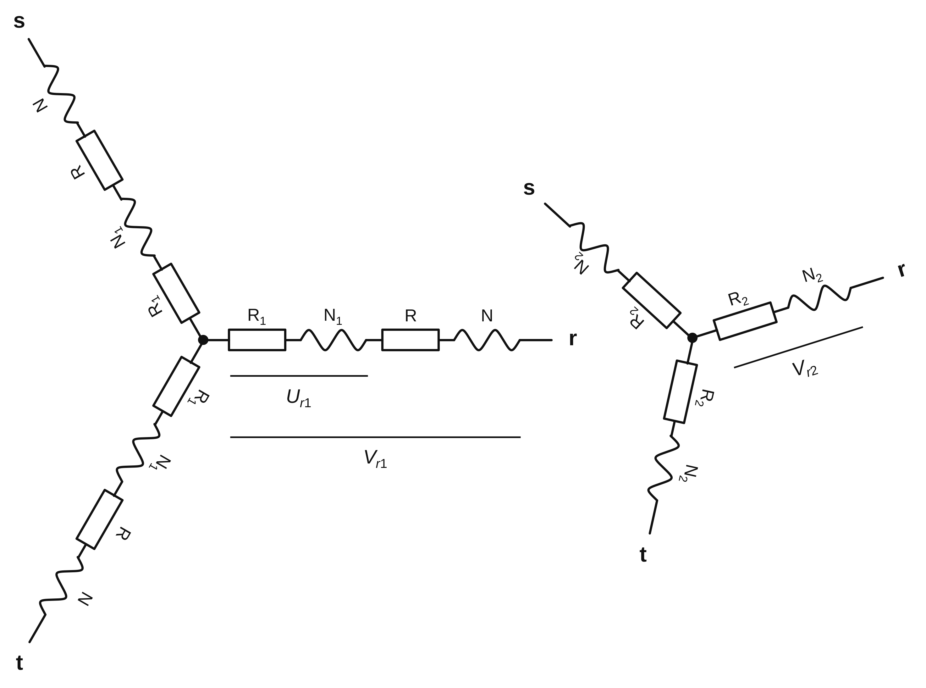
B3.2 dq-transformation
Figure 1 yields expressions for the voltages, which after the dq transformation
\[\begin{bmatrix} \gamma_{d1} \\ \gamma_{q1} \end{bmatrix} = \frac{2}{3} \begin{bmatrix} \sin\theta & \sin\left(\theta-\frac{2\pi}{3}\right) & \sin\left(\theta+\frac{2\pi}{3}\right) \\ \cos\theta & \cos\left(\theta-\frac{2\pi}{3}\right) & \cos\left(\theta+\frac{2\pi}{3}\right) \end{bmatrix} \begin{bmatrix} \gamma_{r1} \\ \gamma_{s1} \\ \gamma_{t1} \end{bmatrix}\]give the following expressions on the stator side:
\[U_{d1} = p\Psi_{d1} - \Psi_{q1}p\theta + (R+R_1)i_{d1},\] \[U_{q1} = p\Psi_{q1} + \Psi_{d1}p\theta + (R+R_1)i_{q1},\]where $\theta$ is the angle between the q-axis and the stator r-axis.
For the rotor, correspondingly ($\beta$ = the angle between the q-axis and the rotor r-axis):
\[\begin{bmatrix} \gamma_{d2} \\ \gamma_{q2} \end{bmatrix} = \frac{2}{3} \begin{bmatrix} \sin\beta & \sin\left(\beta-\frac{2\pi}{3}\right) & \sin\left(\beta+\frac{2\pi}{3}\right) \\ \cos\beta & \cos\left(\beta-\frac{2\pi}{3}\right) & \cos\left(\beta+\frac{2\pi}{3}\right) \end{bmatrix} \begin{bmatrix} \gamma_{r2} \\ \gamma_{s2} \\ \gamma_{t2} \end{bmatrix}\]and
\[U_{d2} = p\Psi_{d2} - \Psi_{q2}p\beta + R_2 i_{d2},\] \[U_{q2} = p\Psi_{q2} + \Psi_{d2}p\beta + R_2 i_{q2}.\]The expressions for the flux linkages are:
\[\Psi_{d1} = (L+L_1+M)i_{d1} + \frac{N_2}{N_1}M i_{d2},\] \[\Psi_{q1} = (L+L_1+M)i_{q1} + \frac{N_2}{N_1}M i_{q2},\] \[\Psi_{d2} = \left(L_2+\frac{N_2}{N_1}M\right)i_{d2} + M i_{d1},\] \[\Psi_{q2} = \left(L_2+\frac{N_2}{N_1}M\right)i_{q2} + M i_{q1},\]when the same dq transformation is used.
To simplify the calculations, it may be convenient to refer the rotor quantities to the stator reference frame. This gives:
\[U'_{d2} = p\Psi'_{d2} - \Psi'_{q2}p\beta + R'_2 i'_{d2},\] \[U'_{q2} = p\Psi'_{q2} + \Psi'_{d2}p\beta + R'_2 i'_{q2},\]where
\[\Psi_{d1} = (L+L_1)i_{d1} + M(i_{d1}+i'_{d2}),\] \[\Psi_{q1} = (L+L_1)i_{q1} + M(i_{q1}+i'_{q2}),\] \[\Psi'_{d2} = L'_2 i'_{d2} + M(i_{d1}+i'_{d2}),\] \[\Psi'_{q2} = L'_2 i'_{q2} + M(i_{q1}+i'_{q2}).\]Here, the relationships
\[i'_2=\frac{N_2}{N_1}i_2,\] \[L'_2=\frac{N_1}{N_2}L_2\]have been used.
Combining these expressions in matrix form gives:
\[\begin{bmatrix} U_{d1} \\ U_{q1} \\ U'_{d2} \\ U'_{q2} \end{bmatrix} = \begin{bmatrix} -\omega(L+L_1+M) & R+R_1+(L+L_1+M)p & -\omega M & Mp \\ R+R_1+(L+L_1+M)p & \omega(L+L_1+M) & Mp & \omega M \\ -(\omega-\omega_r)M & Mp & -(\omega-\omega_r)L'_2 & R'_2+L'_2p \\ Mp & (\omega-\omega_r)M & R'_2+L'_2p & (\omega-\omega_r)L'_2 \end{bmatrix} \begin{bmatrix} i_{d1} \\ i_{q1} \\ i'_{d2} \\ i'_{q2} \end{bmatrix},\]where $\omega_r$ is the angular velocity of the rotor.
Finally, an expression for torque is obtained:
\[M_v = M\left(\frac{a}{2}\right)\left(\frac{P}{2}\right) \left(i_{q1}i'_{d2}-i_{d1}i'_{q2}\right),\]where $a$ is the number of phases and $P$ the number of poles.
B3.3 Fourier Analysis
To continue the analysis, the waveform produced by the inverter is now introduced. The superscript $s$ (for example, $V_{q1}^{s}$) denotes variables in the stator reference system, while $e$ denotes a synchronously rotating reference system.
From the $\gamma$ equations:
\[\begin{aligned} V_{d1}^{s} &= \frac{1}{\sqrt{3}}(-V_{s1}+V_{t1}) \\ &= &= \{\text{Fourier expansion}\} \\ &= \sum_{k=1}^{\infty} \left( V_{kd\alpha}\cos(k\omega_e t) + V_{kd\gamma}\sin(k\omega_e t) \right), \end{aligned}\] \[V_{q1}^{s} = V_{t1} = \sum_{k=1}^{\infty} \left( V_{kq\alpha}\cos(k\omega_e t) + V_{kq\gamma}\sin(k\omega_e t) \right).\]Expressed in the $e$ system, this becomes:
\[V_{d1}^{e} = V_{q1}^{s}\sin(\omega_e t) + V_{d1}^{s}\cos(\omega_e t),\] \[V_{q1}^{e} = V_{q1}^{s}\cos(\omega_e t) - V_{d1}^{s}\sin(\omega_e t).\]Substitution of the expressions for $V_{d1}^{s}$ and $V_{q1}^{s}$ gives forward- and backward-rotating waves, denoted $+e$ and $-e$.
\[\begin{aligned} V_{kd1}^{+e} = \frac{1}{2}\sum_{k=1}^{\infty} \Bigl[ &-(V_{kq\alpha}-V_{kd\gamma}) \sin((k-1)\omega_e t) \\ &+(V_{kq\gamma}+V_{kd\alpha}) \cos((k-1)\omega_e t) \Bigr], \end{aligned}\] \[\begin{aligned} V_{kq1}^{+e} = \frac{1}{2}\sum_{k=1}^{\infty} \Bigl[ &(V_{kq\alpha}-V_{kd\gamma}) \cos((k-1)\omega_e t) \\ &+(V_{kq\gamma}+V_{kd\alpha}) \sin((k-1)\omega_e t) \Bigr], \end{aligned}\] \[\begin{aligned} V_{kd1}^{-e} = \frac{1}{2}\sum_{k=1}^{\infty} \Bigl[ &(V_{kq\alpha}+V_{kd\gamma}) \sin((k+1)\omega_e t) \\ &-(V_{kq\gamma}-V_{kd\alpha}) \cos((k+1)\omega_e t) \Bigr], \end{aligned}\] \[\begin{aligned} V_{kq1}^{-e} = \frac{1}{2}\sum_{k=1}^{\infty} \Bigl[ &(V_{kq\alpha}+V_{kd\gamma}) \cos((k+1)\omega_e t) \\ &+(V_{kq\gamma}-V_{kd\alpha}) \sin((k+1)\omega_e t) \Bigr]. \end{aligned}\]To solve the equations for the different harmonics, it is convenient to establish a separate reference system for each one so that the parameters become constant. The different harmonics are therefore transformed individually:
\[\gamma_{d1}^{+ke} = \gamma_{kq1}^{+e}\sin((k-1)\omega_e t) + \gamma_{kd1}^{+e}\cos((k-1)\omega_e t),\] \[\gamma_{q1}^{+ke} = \gamma_{kq1}^{+e}\cos((k-1)\omega_e t) - \gamma_{kd1}^{+e}\sin((k-1)\omega_e t),\] \[\gamma_{d2}^{+ke} = \gamma_{kq2}^{+e}\sin((k-1)\omega_e t) + \gamma_{kd2}^{+e}\cos((k-1)\omega_e t),\] \[\gamma_{q2}^{+ke} = \gamma_{kq2}^{+e}\cos((k-1)\omega_e t) - \gamma_{kd2}^{+e}\sin((k-1)\omega_e t),\]and
\[\gamma_{d1}^{-ke} = -\gamma_{kq1}^{-e}\sin((k+1)\omega_e t) + \gamma_{kd1}^{-e}\cos((k+1)\omega_e t),\] \[\gamma_{q1}^{-ke} = \gamma_{kq1}^{-e}\cos((k+1)\omega_e t) + \gamma_{kd1}^{-e}\sin((k+1)\omega_e t),\] \[\gamma_{d2}^{-ke} = -\gamma_{kq2}^{-e}\sin((k+1)\omega_e t) + \gamma_{kd2}^{-e}\cos((k+1)\omega_e t),\] \[\gamma_{q2}^{-ke} = \gamma_{kq2}^{-e}\cos((k+1)\omega_e t) + \gamma_{kd2}^{-e}\sin((k+1)\omega_e t).\]With the rotor voltages equal to zero, combining the equations above gives:
\[V_{d1}^{+ke} = \frac{1}{2}(V_{kq\alpha}+V_{kd\gamma}),\] \[V_{q1}^{+ke} = \frac{1}{2}(V_{kq\gamma}-V_{kd\alpha}),\] \[V_{d1}^{-ke} = \frac{1}{2}(V_{kq\alpha}-V_{kd\gamma}),\] \[V_{q1}^{-ke} = \frac{1}{2}(V_{kq\alpha}+V_{kd\gamma}).\]The currents can now be solved by taking the inverse of
\[\begin{bmatrix} V_{d1} \\ V_{q1} \\ 0 \\ 0 \end{bmatrix}^{\pm ke} = \begin{bmatrix} -n\omega_e(L+L_1+M) & R+R_1+(L+L_1+M)p & -n\omega_eM & Mp \\ R+R_1+(L+L_1+M)p & n\omega_e(L+L_1+M) & Mp & n\omega_eM \\ -(n\omega_e-\omega_r)M & Mp & -(n\omega_e-\omega_r)L'_2 & R'_2+L'_2p \\ Mp & (n\omega_e-\omega_r)M & R'_2+L'_2p & (n\omega_e-\omega_r)L'_2 \end{bmatrix} \begin{bmatrix} i_{d1} \\ i_{q1} \\ i'_{d2} \\ i'_{q2} \end{bmatrix}^{\pm ke}\]These are solved and then yield losses and torque in the usual manner from the conventional equivalent circuit for the forward- and backward-rotating waves.
Appendix B4. Program Description: PWMIND
Table of Contents
B4.1 $\ $ General
B4.2 $\ $ Scope of Application
B4.3 $\ $ Calculation Sequence
B4.4 $\ $ Input Data
B4.5 $\ $ Output
B4.6 $\ $ “Constant Flux”
B4.7 $\ $ “s Iteration”
B4.8 $\ $ Operating Instructions
B4.9 $\ $ Program Listing
B4.10 $\ $ Run Example
B4.1 General
The PWMIND program is a modification of the PWMOT program and calculates losses, voltage, current, and torque for an arbitrary combination of a series inductor and an induction machine.
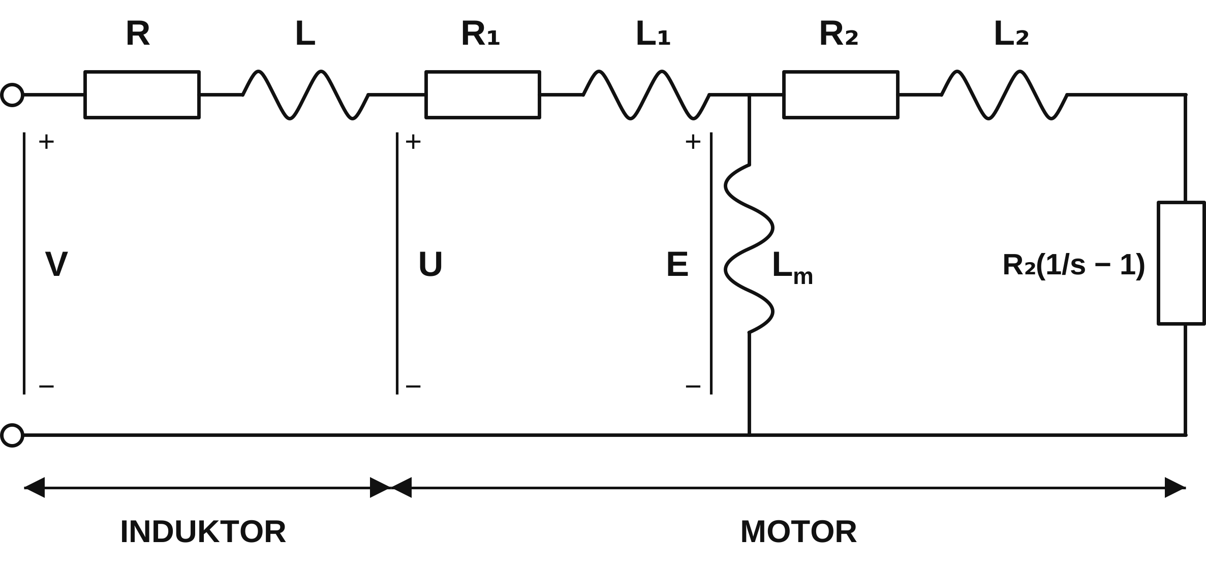
B4.2 Scope of Application
Correct results are obtained for all linear equivalent circuits in which the supply voltage has an arbitrary waveform and frequency. The program also accounts for current displacement, which becomes significant especially at high frequencies.
B4.3 Calculation Sequence
The program first performs a Fourier analysis of the voltage. It then calculates the currents for each harmonic from the machine data and the voltage amplitude. These results are finally used to obtain the voltage drop across the inductor and the losses, torque, and voltage drop in the motor.
B4.4 Input Data
The voltage input data are requested first:
| Program variable | Quantity | Reference |
|---|---|---|
| $N$ | $J’$ | Appendix 2 |
| AIN(I) | $\alpha_i$ | Appendix 2 |
| $\mathrm{NMAX}$ | Highest term in the Fourier expansion | |
| APK | $m$ | Appendix 2 |
| MK | $p$ | Appendix 2 |
| FFT | $\theta_0$ | Appendix 2 |
Alternatively, the coefficients of selected harmonics can be obtained by continuous Fourier expansion (IS, NRWANT(I)).
For constant flux, see the section under that heading.
The machine parameters are entered next. This needs to be done only before the first calculation or when new machine data are required.
| Program variable | Meaning | Unit/remark |
|---|---|---|
| RES(1) | Stator resistance | $\Omega/\text{phase}$, equivalent Y |
| XI(1) | Stator reactance | Same |
| XI(2) | Magnetizing reactance | Same |
| XI(3) | Rotor reactance | Same |
| RES(2) | Rotor resistance | Same |
| POLES | Number of poles | — |
| BASEF | Base frequency | Hz |
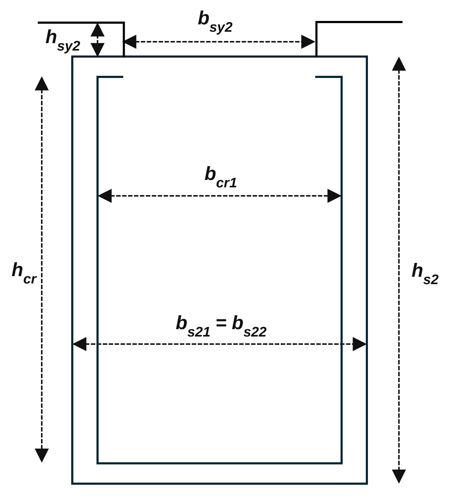
The labels in the figure denote:
SPTR: slot type according to the RESIST program $\rho_2$: conductor resistivity- $R_{\mathrm{rat}}$: ratio of the slot mean diameter to the rotor mean diameter
The above shows the rotor-slot dimensions required for calculating current displacement.
For s iteration, see the section under that heading.
The following are also required to start the calculation:
| Program variable | Meaning | Unit |
|---|---|---|
FM0 |
Current frequency | Hz |
SM |
Slip | |
UD/2 |
Half the DC-link voltage | V |
For the series inductor, the following are required:
| Program variable | Meaning | Unit |
|---|---|---|
R |
Inductor resistance | $\Omega/\text{phase}$ |
L |
Inductor inductance | H/phase |
B4.5 Output
The output values are self-explanatory, but note that the voltages are peak values.
B4.6 “Constant Flux”
When the induction machine is used at different frequencies, constant flux $\Phi$ is always sought in order to minimize losses at constant load torque. This flux $\Phi$ is proportional to $E/f$; consequently, for constant flux, $E$ should be kept linearly proportional to frequency (for the fundamental). Because voltage drops occur across the inductor and stator impedances, the terminal voltage $V$ must be increased continuously to maintain constant flux. This is most noticeable at low frequencies.
$V$ is raised by increasing the pulse ratio above its normal value of
\[\mathrm{APK}=\frac{\mathrm{FM0}}{\mathrm{FB}}.\]In this way, the modulation signal becomes wider and the peak value of the fundamental increases. This can be maintained only at low frequencies and small inductances, however, because otherwise the pulse ratio becomes greater than one, which is impossible.
To hold the flux constant, the question is therefore answered with a one. The program then enters an iterative loop between 0800 and 3060. The loop begins by calculating the Fourier terms. The peak value of the fundamental flux voltage EQ (= the program’s flux voltage) is then calculated. If it differs from the desired peak value E1 of the flux voltage, execution returns to 103 and the pulse ratio APK is changed.
The iteration continues in this way until EQ and E1 differ by no more than 0.4%. The loop is then exited, and the program continues normally using the most recently applied pulse ratio.
NOTE: $E$ is a peak value.
B4.7 “s Iteration”
At sufficiently high frequencies or inductances, the flux cannot be held constant. The slip must instead be increased to obtain constant torque.
To determine the slip required for a given torque, an iterative loop has been inserted between 1920 and 3140. If the s-iteration question is answered yes, this loop is executed for the fundamental. At 3140, the fundamental torque ($\approx$ total torque) is output. If it differs from the desired torque, the loop is entered again with a different s value.
Warning. Because the loops interact, care is required. If, for example, a constant-flux iteration is performed, it is inadvisable to enter the s-iteration loop at the same time.
B4.8 Operating Instructions
The program is designed for TIME SHARING and is therefore run from a terminal. After logging in, enter:
FORT
RUN CPWMIND;CSUBROUT
to which the terminal responds:
LOADER DIAGNOSTICS ......
The program then requests the parameters described as input data in Section 4.
Further information can be obtained from the program description for PWMOT.
B4.9 Program Listing: PWMIND
Part 1
0100C     PROGRAM FÖR MASKINBERÄKNING MED PWM REFERENS-
0110C     OCH MODULATIONSPULSER SOM INDATA
0120C     PROGRAMMET BERÄKNAR MOMENTANVÄRDEN PÅ SPÄNNING,
0130C     STRÖMMAR OCH MOMENT. FÖRLUSTER BERÄKNAS
0140C     *******************************************************
0150      DIMENSION RES(50,5),AIN(10),NRWANT(50)
0155      DIMENSION KIND(50),IIND(50)
0160      DIMENSION ABM(50,5),U(50,2,2)
0165      DIMENSION UDQ(50),UDG(50),UDA(50), VOD(50)
0170      DIMENSION DELTAU(50,2)
0180      DIMENSION VOD(50,4),HM(20),EE(4),SI(4),BS(20)
0190      DIMENSION AINTID(10)
0200      DIMENSION H(20),BC(20),RHO(20)
0210      DIMENSION A(50,2,4),RROT(50,2),EFF(50,2)
0220      COMMON/LABEL2/RS,LS,M,LR,RR,WE,WR,A(4,4),RI,LI,B(4,4)
0230      COMMON/LABEL1/IND(199)
0240      REAL PI/3.14159/
0250      REAL MOM1
0260      REAL KM,LS,LR,M,LI
0270      REAL PCU1,PCU2,IQST,IDST,IQRT,IDRT,MOMT
0280      CHARACTER TEXT*42
0290    1 CONTINUE
0300      DO 3 I=1,50
0310      NRWANT(I)=0
          KIND(I)=0
          IIND(I)=0
0320      IF(I.LT.11) AIN(I)=0.
0330    3 CONTINUE
0340      DO 5 I=2,198,2
0350      IND(I)=3*I-1
0360    5 IND(I+1)=3*I+1
0370      IND(1)=1
0380      PRINT,"GE ANTAL ARGUMENT (ALFA) SOM INTE=0"
0390      READ,N
0400      NTID=N
0410      PRINT,"GE ARGUMENTEN I GRADER"
0420      READ,(AINTID(I),I=1,N)
0430      DO 10 I=1,N
0440   10 AIN(I)=AINTID(I)*PI/180
0450      DO 7 I=1,N
0460      AINTID(I)=AIN(I)
0470    7 CONTINUE
0480      PRINT,"ÖNSKAS SÄRSKILDA FREKVENSER? 1=JA"
0490      READ,IS
0500      IF(IS.NE.1) GO TO 15
0510      PRINT,"GE ANTALET ÖNSKADE FREKVENSER"
0520      READ,NT
0530      PRINT,"GE FREKVENSERNA SOM F/F0, F0=GRUNDTON"
0540      READ,(NRWANT(I),I=1,NT)
0550      GO TO 40
0560   15 PRINT,"GE HÖGSTA ÖNSKADE FREKVENS F/F0, F0=GRUNDTON"
0570      READ,NMAX
0580      DO 20 I=1,199
0590      IF(IND(I).GT.NMAX) GO TO 30
0600   20 NRWANT(I)=IND(I)
0610   30 NT=I-1
0620   40 CONTINUE
0630      PRINT,"GE PULSKVOT"
0640      READ,APK
0650      PRINT,"GE (ANTALET PULSER PER PERIOD)/6"
0660      READ,MK
0670      MKN=6*MK
0680      PRINT,"GE FASFÖRSKJUTNING I GRADER"
0690      READ,FFI
Part 2
0700      PRINT,"GE MINSTA AMPLITUD SOM SKALL ADDERAS"
0710      READ,RMMIN
0720      FFI=FFI*PI/180
0730      IE=2
0740      PRINT,"ÖNSKAS KONSTANT FLÖDE? 1=JA"
0750      READ,IE
0760      IF(IE.NE.1) GOTO 107
0770      PRINT,"GE ÖNSKAT E-VÄRDE"
0780      READ,E1
0790  107 CONTINUE
0800  103 CONTINUE
0810C
0820      WRITE(6,104) APK
0830  104 FORMAT(1X,"PULSKVOT=",F10.4)
0840      K1=0
0850      N=NTID
0860      DO 109 I=1,N
0870  109 AIN(I)=AINTID(I)
0880      DO 200 J=1,NT
0890      R1=APK*REFK(N,AIN,NRWANT(J))
0900      R2=NRWANT(J)
0910      R3=0
0920      CALL FIND1(NRWANT(J),MKN,KIND,IIND,M1)
0930      IF(M1.LT.1) GO TO 120
0940      DO 110 J1=1,M1
0950      RM=AMT(APK,IIND(J1))*REFK(N,AIN,KIND(J1))/2.
0960      FI=-IIND(J1)*FFI
0970      IF(ABS(RM).LT.RMMIN) GO TO 110
0980      CALL ADD(RM,R1,FI,R3,FI,RR1,RR3)
0990      R1=RR1
1000      R3=RR3
1010  110 CONTINUE
1020  120 CONTINUE
1030      CALL FIND2(NRWANT(J),MKN,KIND,IIND,M2)
1040      IF(M2.EQ.0) GO TO 150
1050      DO 140 J2=1,M2
1060      K2=IABS(KIND(J2))
1070      I2=IABS(IIND(J2))
1080      RM=AMT(APK,I2)*REFK(N,AIN,K2)/2.
1090      RM=RM*SIGN(1.,KIND(J2))
1100      IF(ABS(RM).LT.RMMIN) GO TO 140
1110      FI=FFI*IIND(J2)
1120      CALL ADD(RM,R1,FI,R3,FI,RR1,RR3)
1130      R1=RR1
1140      R3=RR3
1150  140 CONTINUE
1160  150 K1=K1+1
1170      RES(K1,1)=R1
1180      RES(K1,2)=R2
1190      RES(K1,3)=R3
1200  200 CONTINUE
1210C
1220      IF(IE.EQ.1) GOTO 411
1230      WRITE(6,420)
1240  420 FORMAT(1X,5(1H*),/T10,"RESULTAT AV FOURIERANALYS:",
         &    /5(1H*),/T10,"F/F0",5X,"AMPLITUD",3X,"FASVINKEL",
         &    /70(1H-))
1260      WRITE(6,430)(RES(I,2),RES(I,1),RES(I,3),I=1,K1)
1270  430 FORMAT(1X,T10,F4.0,5X,F7.5,2X,F9.5)
1280  440 CONTINUE
1290  411 CONTINUE
Part 3
1300      PRINT,"ÖNSKAS NY FOURIER-ANALYS ? 1=JA"
1310      READ,IIVS
1320      IF(IIVS.EQ.1) GO TO 1
1330      PRINT,"NYA MASKINKONSTANTER ? 1=JA"
1340      READ,MASK
1350C
1360      K3=K1
1370      IF(MASK.NE.1) GOTO 405
1380      PRINT,"ÖNSKAS MBK 280 S-6:S MASKINKONSTANTER? 1=JA"
1390      READ,IMBK
1400      IF(IMBK.NE.1) GOTO 404
1410      RS=.048
          XLS=.21
          XM=3.886
          XLR=.16
          RRO=.051
          P=6
          FB=50
1420      SPTR=2
          BS21=3.95
          BS22=3.95
          HS2=29.2
          BSY2=2
          HSY2=1
1430      BSMR=0
          HSMR=0
          BCR1=3.75
          BCMR=0
          HCR=28
          RHO2=.0425
          RRAT=.65
1440  404 CONTINUE
1450      IF(IMBK.EQ.1) GOTO 405
1460      PRINT,"GE INDATA: RS,XLS,XM,XLR,RRO,P,FB"
1470      READ,RS,XLS,XM,XLR,RRO,P,FB
1480      PRINT,"ROTOR-SPTR: BS21,BS22,HS2,BSY2,HSY2,BSMR,HSMR",
1490     &    " BCR1,BCMR,HCR,RHO2,RRAT"
1500      READ,SPTR,BS21,BS22,HS2,BSY2,HSY2,BSMR,HSMR,
1510     &    BCR1,BCMR,HCR,RHO2,RRAT
1520  405 CONTINUE
1530      PRINT,"ÖNSKAS S-ITERATION? 1=JA"
1540      READ,IIVS
1550  390 PRINT,"GE FM0, SM, UD/2"
1560      READ,FM0,SM,UM1
1570      RI=0
          LI=0
1580      PRINT,"SKALL SERIEREAKTOR INGÅ I BERÄKNINGARNA? 1=JA"
1590      READ,KS
1600      IF(KS.NE.1) GOTO 392
1610      PRINT,"GE SERIEREAKTORDATA: R,L"
1620      READ,RI,LI
1630      XL=2*PI*FB*LI
1640  392 CONTINUE
1650  397 CONTINUE
1660  394 CONTINUE
1670      CALL SARE(SPTR,BS21,BS22,HS2,BSY2,HSY2,BSMR,HSMR,
1680     &    BCR1,BCMR,HCR,RHO2,N,BS,H,BC,RHO)
1690      WRITE(6,530)
1700  530 FORMAT(1X,5(1H*))
1710C     UPPLÄGGNING AV RESULTAT FRÅN FOURIER-ANALYS
1720C     3-FAS TILL Q OCH D-AXEL
1730      WRITE(6,545)
1740C
1750      K1=K3
1760      IF(IIVS.EQ.1) K1=1
1770      IF(IE.EQ.1) K1=1
1780      DO 540 I=1,K1
1790      A2=RES(I,1)*SIN(RES(I,3))+UM1
1800      B3=RES(I,1)*COS(RES(I,3))+UM1
1810      ABM(I,1)=RES(I,2)
1820      ABM(I,2)=A2
1830      ABM(I,3)=B3
1840      IN=ABM(I,1)
1850  540 WRITE(6,550) A2,IN,B3,IN
1860C
1870      PRINT,"COPY"
          READ,STRUNT
1880  545 FORMAT(1X,6(1H*),/T10,"SPÄNNING Q-AXEL")
1890  550 FORMAT(1X,T10,F10.3,"*COS(",I2,"*WT) +",
Part 4
1900     &    I2,"*WT) + ",F10.3,"*SIN(",I2,"*WT) +")
1910  559 CONTINUE
1920      WRITE(6,530)
1930C     WQ & WD
1940      S2=2/SQRT(3)
1950C
1960      K1=K3
1970      IF(IIVS.EQ.1) K1=1
1980      IF(IE.EQ.1) K1=1
1990      DO 560 I=1,K1
2000      ABM(I,4)=S2*ABM(I,3)*SIN(ABM(I,1)*2*PI/3)
2010      ABM(I,5)=-S2*ABM(I,2)*SIN(ABM(I,1)*2*PI/3)
2020      IN=ABM(I,1)
2030  560 CONTINUE
2040C
2050      XS=XLS+XM
2060      XR=XLR+XM
2070      WP=2*PI*FB
2080      WE=2*PI*FM0
2090      LS=XS/WP
2100      M=XM/WP
2110C
2120      EE(3)=0.
2130      EE(4)=EE(3)
2140C
2150      IF(KS.NE.1) GOTO 699
2160      DO 698 K=1,50
2170      DO 698 J=1,2
2180      DO 698 I=1,2
2190      U(K,J,I)=0.0
2200  698 CONTINUE
2210  699 CONTINUE
2220      K1=K3
2230      IF(IE.EQ.1) K1=1
2240      DO 700 K=1,K1
2250      KU=ABM(K,1)
2260      WR=WE*(1-SM)
2270C
2280      VOD(K,1)=0.5*(ABM(K,2)-ABM(K,5))
2290      VOD(K,2)=0.5*(ABM(K,3)+ABM(K,4))
2300      VOD(K,3)=0.5*(ABM(K,2)+ABM(K,5))
2310      VOD(K,4)=0.5*(ABM(K,3)-ABM(K,4))
2320C
2330      DO 700 J=1,3,2
2340      MP=1
2350      IF(J.EQ.3) MP=2
2360      EE(1)=VOD(K,J)
2370      EE(2)=VOD(K,J+1)
2380      KW=ABM(K,1)
2390      IF(J.EQ.3) KW=-ABM(K,1)
2400      F2=ABS(KW*WE-WR)/(2*PI)
2410      CALL RSPIMP(1,F2,N,0,BS,H,BC,RHO,
         &    Z1,Z2,Z3,Z4,Z5,Z6,Z7,Z8)
2420      CALL RSPIMP(1,.1,N,0,BS,H,BC,RHO,
         &    Z3,Z4,Z5,Z6,Z7,Z8,Z9,Z10)
2430      RFACT=RRAT*(Z1/Z3-1.0)+1.0
2440      XFACT=RRAT*(Z2*.1/(Z4*F2)-1.0)+1.0
2450      LR=(XLR*XFACT+XM)/WP
2460      RR=RRO*RFACT
2470      RROT(K,MP)=RR
2480      CALL SETA(KW)
2490      CALL MINF(F2,4,4,0.0001,HM,IER2)
Part 5
2500      DO 620 I=1,4
2510      SUM=0.0
2520C
2530      DO 630 J2=1,4
2540      SUM=SUM+H(I,J2)*EE(J2)
2550  630 CONTINUE
2560C
2570      SI(I)=SUM
2580      IF(KB.NE.1) GOTO 632
2590      DO 631 J3=1,2
2600      U(K,MP,J3)=B(J3,I)*SI(I)+U(K,MP,J3)
2610  631 CONTINUE
2620  632 CONTINUE
2630  620 CONTINUE
2640C     STRÖMMAR I Q&D-PLANET
2650C
2660      DO 700 I=1,4
2670      AI(K,MP,I)=SI(I)
2680  700 CONTINUE
2690C
2700      IF(KB.NE.1) GOTO 702
2710      K1=K3
2720      IF(INYS.EQ.1) K1=1
2730      IF(IE.EQ.1) K1=1
2740      DO 701 K=1,K1
2750      UDA(K)=U(K,1,1)+U(K,2,1)
2760      UDG(K)=U(K,1,2)+U(K,2,2)
2770      UDA(K)=U(K,1,2)-U(K,2,2)
2780      UDG(K)=U(K,2,1)-U(K,1,1)
2790      DELTAU(K,1)=ABM(K,2)-UDA(K)
2800      DELTAU(K,2)=ABM(K,3)-UDG(K)
2810  701 CONTINUE
2820  702 CONTINUE
2830C
2840C
2850C     EFFEKTFÖRLUSTER I STATOR OCH ROTOR:
2860      PCU1=0
2870      PCU2=0
2880C
2890      K1=K3
2900      IF(INYS.EQ.1) K1=1
2910      IF(IE.EQ.1) K1=1
2920      DO 710 K=1,K1
2930      APCU1=RS*1.5*(AI(K,1,1)**2+AI(K,1,2)**2)
2940      BPCU1=RS*1.5*(AI(K,2,1)**2+AI(K,2,2)**2)
2950      EFF(K,1)=APCU1+BPCU1
2960      IF(IE.NE.1) GOTO 705
2970  742 CONTINUE
2980      DENOM=(RRO/SM)**2+((XLR+XM)*FM0/FB)**2
2990      RH=RRO/SM*(XM*FM0/FB)**2/DENOM
3000      XH=((RRO/SM)**2*XM*FM0/FB+
         &     XLR*XM*(XLR+XM)*(FM0/FB)**3)/DENOM
3010      EQ=RES(1,1)*UM1*SQRT((RH**2+XH**2)/((RI+RS+RH)**2
3020     &     +(XL*FM0/FB+XLS*FM0/FB+XH)**2))
3030      IF(INYS.EQ.1) GOTO 748
3040      APK1=APK
3050      APK=APK*E1/EQ
3060      IF(ABS((EQ-E1)/E1).GT.0.004) GOTO 103
3070  748 CONTINUE
3080      WRITE(6,713)EQ
3090  713 FORMAT(1X,"EQ=",F13.3)
Part 6
3100      CPCU2=1.5*RROT(1,1)*(AI(1,1,3)**2+AI(1,1,4)**2)
3110      DPCU2=1.5*RROT(1,2)*(AI(1,2,3)**2+AI(1,2,4)**2)
3120      MOM1=P*(CPCU2+DPCU2)/SM/4/PI/FM0
3130      WRITE(6,712)MOM1
3140  712 FORMAT(1X,"MOMENTET=",F13.3,"
         &   ÖNSKAS NY ITERATION? 1=JA")
3150      IF(INYS.EQ.1) GOTO 405
3160      READ,INY
3170      IF(INY.NE.1) GOTO 704
3180      GOTO 390
3190  704 IE=2
          APK=APK1
3200      GOTO 103
3210  705 CONTINUE
3220      IF(INYS.EQ.1) GOTO 742
3230      INYS=2
3240      BPCU2=1.5*RROT(K,2)*(AI(K,2,3)**2+AI(K,2,4)**2)
3250      APCU2=1.5*RROT(K,1)*(AI(K,1,3)**2+AI(K,1,4)**2)
3260      EFF(K,2)=APCU2+BPCU2
3270C
3280      IT=ABM(K,1)
3290      WRITE(6,720)K,IT,EFF(K,1),EFF(K,2),RROT(K,1),RROT(K,2)
3300      PCU1=PCU1+EFF(K,1)
3310      PCU2=PCU2+EFF(K,2)
3320  710 CONTINUE
3330      AIP1=SQRT(PCU1/(3*RS))
3340      PRINT,"COPY"
          READ,STRUNT
3350      WRITE(6,730)PCU1,PCU2,AIP1
3360  720 FORMAT(1X,"K=",I2," F/F0=",I2," PCU1=",F7.1,
3370     &    " PCU2=",F7.1," R2+=",E10.3," R2-=",E10.3//)
3380  730 FORMAT(1X,70(1H-),//,T10,"SUMMA PCU1=",E11.4," W",
3390     &    /T10,"SUMMA PCU2=",E11.4," W",
3400     &    /T10,"I1     =",E11.4," A",/70(1H-))
3410      IF(KB.NE.1) GOTO 737
3420      PRINT,"SPÄNNINGSFALL ÖVER REAKTORN"
3430      PRINT,"    Q-AXELN"
3440      PRINT,"    +COS(NWT)    +SIN(NWT)"
3450      DO 736 K=1,K1
3460      WRITE(6,734)DELTAU(K,1),DELTAU(K,2)
3470  734 FORMAT(1X,2F12.4)
3480  736 CONTINUE
3490  737 CONTINUE
3500C     MOMENTBERÄKNINGAR
3510      AMVM=0
          AMOMA=-1E8
          AMOMI=1E8
3520      T=1/(FM0*MK)
3530      T1=T/50
3540      TI=0
          NTM=0
3550C
3560  735 CONTINUE
3570      IF(TI.GT.T) GOTO 750
3580      IQST=0
          IDST=0
          IQRT=0
          IDRT=0
3590      DO 740 K=1,K1
3600      FI=ABM(K,1)*(WE*TI-PI/6.)
3610C     STATORSTRÖM:
3620      IQST=IQST+(AI(K,1,1)+AI(K,2,1))*COS(FI)
3630     &    +(AI(K,1,2)-AI(K,2,2))*SIN(FI)
3640      IDST=IDST+(AI(K,1,2)+AI(K,2,2))*COS(FI)
3650     &    -(AI(K,1,1)-AI(K,2,1))*SIN(FI)
3660C     ROTORSTRÖM:
3670      IQRT=IQRT+(AI(K,1,3)+AI(K,2,3))*COS(FI)
3680     &    +(AI(K,1,4)-AI(K,2,4))*SIN(FI)
3690      IDRT=IDRT+(AI(K,1,4)+AI(K,2,4))*COS(FI)
Part 7
3700 & -(AI(K,1,3)-AI(K,2,3))*SIN(FI)
3710 740 CONTINUE
3720C
3730 MOMT=M*0.75*P*(IQST*IDRT-IDST*IQRT)
3740 AMVM=AMVM+MOMT
3750 IF(MOMT.GT.AMOMA)AMOMA=MOMT
3760 IF(MOMT.LT.AMOMI)AMOMI=MOMT
3770 TI=TI+T1
3780 NTM=NTM+1
3790 GO TO 735
3800 750 CONTINUE
3810 AMVM=AMVM/NTM
3820 AMVAR1=AMOMA-AMVM
3830 AMVAR2=AMOMI-AMVM
3840 WRITE(6,760)T,AMVM,AMVAR1,AMVAR2
3850 760 FORMAT(1X,/70(1H-),/T10,"MOMENTET UNDER",E11.4,
& " SEK. :",
3860 & /T10,"MEDELVÄRDE:",E11.4," NM",
3870 & /T10,"AMPLITUD :",E11.4," NM",
3880 & /T10,"AMPLITUD :",E11.4," NM",/70(1H-))
3890C ÖGONBLICKSVÄRDEN: STRÖM, SPÄNNING OCH MOMENT
3900 805 CONTINUE
3910 PRINT,"ÖNSKAS PLOT ELLER TABELL? 1=PLOT 2=TABELL"
3920 READ,LP
3930 PRINT,"GE TEXT TILL TABELL ELLER PLOT"
3940 READ,TEXT
3950 PRINT,"GE TIDSINTERVALL FÖR PLOT ELLER UTSKRIFT"
3960 PRINT,"T1<T<T2 MILLISEC. ; T1>=0"
3970 READ,T1,T
3980 T1=T1/1000
3990 T=T/1000
4000 PRINT,"GE ANTALET STEG I INTERVALLET"
4010 READ,STEG
4020 TD=(T-T1)/STEG
4030 IF(LP.EQ.2)GOTO 808
4040 PRINT,"GE AMPLITUDER FÖR SKALNING !"
4050 PRINT,"SPÄNNING (V),STATORSTRÖM (A), MOMENT (NM)"
4060 READ,UMAX,AIQSMAX,AMOMAX
4070 CALL PLOTS
4080 CALL ERASE
4090 WRITE(6,940)TEXT
4100 CALL FRAME(0.,0.,16.,14.,2)
4110 DX=(T-T1)/10.
4120 CALL AXIS(4.,1.,"TID (SEKUNDER) ",-15,10.,0.,T1,DX)
4130 DY1=2*UMAX/10.
4140 CALL AXIS(1.,1.,"SPÄNNING (V)",15,10.,90.,
& -UMAX,DY1)
4150 DY2=2*AIQSMAX/10.
4160 CALL AXIS(2.,1.,"STATORSTRÖM (A)",15,10.,90.,
& -AIQSMAX,DY2)
4170 DY3=2*AMOMAX/10.
4180 CALL AXIS(3.,1.,"MOMENT (NM)",15,10.,90.,
& -AMOMAX,DY3)
4190 CALL PLOT(4.,6.,23)
4200 GO TO 810
4210 808 CONTINUE
4220 WRITE(6,930)TEXT
4230 WRITE(6,910)
4240C
4250 810 CONTINUE
4260 IF(TI.GT.T)GO TO 905
4270 IQST=0
IDST=0
IQRT=0
IDRT=0
UDST=0
4280C
4290 DO 900 K=1,K1
Part 8
4300      FI=ABM(K,1)*(WE*TI-PI/6.)
4310      FI1=ABM(K,1)*WE*TI
4320C     STATORSTRÖM:
4330      IQST=IQST+(AI(K,1,1)+AI(K,2,1))*COS(FI)
4340     &    +(AI(K,1,2)-AI(K,2,2))*SIN(FI)
4350      IDST=IDST+(AI(K,1,2)+AI(K,2,2))*COS(FI)
4360     &    -(AI(K,1,1)-AI(K,2,1))*SIN(FI)
4370C     ROTORSTRÖM:
4380      IQRT=IQRT+(AI(K,1,3)+AI(K,2,3))*COS(FI)
4390     &    +(AI(K,1,4)-AI(K,2,4))*SIN(FI)
4400      IDRT=IDRT+(AI(K,1,4)+AI(K,2,4))*COS(FI)
4410     &    -(AI(K,1,3)-AI(K,2,3))*SIN(FI)
4420      UDST=UDST+ABM(K,4)*COS(FI1)+ABM(K,5)*SIN(FI1)
4430  900 CONTINUE
4440C
4450      UDST=UDST*SQRT(3)
4460      MOMT=M*0.75*P*(IQST*IDRT-IDST*IQRT)
4470C     UTSKRIFT I TABELL
4480      IF(LP.EQ.2)GO TO 902
4490      CALL PLOT(TI/DX,UDST/DY1,3)
4500      CALL PLOT(TI/DX,UDST/DY1,2)
4510      CALL PLOT(TI/DX,IDST/DY2,3)
4520      CALL PLOT(TI/DX,IDST/DY2,2)
4530      CALL PLOT(TI/DX,MOMT/DY3,3)
4540      CALL PLOT(TI/DX,MOMT/DY3,2)
4550      GO TO 904
4560  902 F10=WE*TI
4570      WRITE(6,920)TI*1000,F10,MOMT,UDST,IDST,IDRT
4580  904 TI=TI+TD
4590      GO TO 810
4600  905 CONTINUE
4610      IF(LP.EQ.2)GO TO 908
4620      CALL HDCOPY
4630      DO 906 NNM=1,5
4640  906 CALL BELL
4650      READ,STRUNT
4660      CALL PLOT(0.,0.,23)
4670      CALL ERASE
4680      CALL ENDP
4690  908 CONTINUE
4700      WRITE(6,530)
4710      PRINT,"ÖNSKAS NY UTSKRIFT (PLOT) ? 1=JA"
4720      READ,ISVAR
4730      IF(ISVAR.EQ.1)GO TO 805
4740  910 FORMAT(1X,70(1H-),/T9,T15,"W0*T",T25,"M",T35,"U",
4750     &    T45,"I1",T55,"I2",//"(MS)",T11,"(RAD)",T25,"(NM)",
4760     &    T35,"(V)",T45,"(A)",T55,"(A)",/70(1H-))
4770  920 FORMAT(1X,F8.3,T15,F6.4,T25,F7.2,T35,F7.1,T45,F7.1,
         &    T55,F7.1)
4780  930 FORMAT(1X,70(1H-),/T10,A30)
4790  940 FORMAT(1X,T20,A30)
4800 1000 CONTINUE
4810      PRINT,"ÖNSKAS NY MASKINBERÄKNING? 1=JA"
4820      READ,MASKIN
4830      IF(MASKIN.EQ.1)GO TO 440
4840      PRINT,"ÖNSKAS NY KÖRNING? 1=JA"
4850      READ,ISLUT
4860      IF(ISLUT.EQ.1)GO TO 1
4870      STOP
          END
Part 9
5650      SUBROUTINE SETA(N)
5660      COMMON/LABEL2/RS,LS,M,LR,RR,WE,WR,A(4,4),RI,LI,B(4,4)
5670      REAL M,LS,LR,LI
5680C
5690      A(1,1)=RS+RI
5700      A(1,2)=N*WE*(LS+LI)
5710      A(1,3)=0.0
5720      A(1,4)=N*WE*M
5730      A(2,1)=-N*WE*(LS+LI)
5740      A(2,2)=RS+RI
5750      A(2,3)=-N*WE*M
5760      A(2,4)=0.0
5770      A(3,1)=0.0
5780      A(3,2)=(N*WE-WR)*M
5790      A(3,3)=RR
5800      A(3,4)=(N*WE-WR)*LR
5810      A(4,1)=-(N*WE-WR)*M
5820      A(4,2)=0.0
5830      A(4,3)=-(N*WE-WR)*LR
5840      A(4,4)=RR
5841      B(1,1)=RS
5842      B(1,2)=N*WE*LS
5843      B(2,1)=-N*WE*LS
5844      B(2,2)=RS
5845      DO 2 J=3,4
5846      DO 2 I=3,4
5847      B(I,J)=A(I,J)
5848    2 CONTINUE
5849      B(1,3)=A(1,3)
5850      B(1,4)=A(1,4)
5851      B(2,3)=A(2,3)
5852      B(2,4)=A(2,4)
5853      B(3,1)=A(3,1)
5854      B(3,2)=A(3,2)
5855      B(4,1)=A(4,1)
5856      B(4,2)=A(4,2)
5857      RETURN
5860      END
Appendix 4.10 Run Example
B4.10.1 Input Data and Initial Iterations
GE ANTAL ARGUMENT (ALFA) SOM INTE=0
=0

GE ARGUMENTEN I GRADER
=0

ÖNSKAS SÄRSKILDA FREKVENSER? 1=JA
=2

GE HÖGSTA ÖNSKADE FREKVENS F/F0, F0=GRUNDTON
=53

GE PULSKVOT
=.67

GE (ANTALET PULSER PER PERIOD)/6.
=2

GE FASFÖRSKJUTNING I GRADER
=0

GE MINSTA AMPLITUD SOM SKALL ADDERAS
=1E-10

ÖNSKAS KONSTANT FLÖDE? 1=JA
=1

GE ÖNSKAT E-VÄRDE
=170

PULSKVOT=    0.6700

ÖNSKAS NY FOURIER-ANALYS? 1=JA
=2

NYA MASKINKONSTANTER? 1=JA
=1

ÖNSKAS MBK 280 S-6:S MASKINKONSTANTER? 1=JA
=1

ÖNSKAS S-ITERATION? 1=JA
=2

GE FM0, SM, UD/2
=30 .0525 244

SKALL SERIEREAKTOR INGÅ I BERÄKNINGARNA? 1=JA
=1

GE SERIEREAKTORDATA:R,L
=.006 .001
The first calculated fundamental component of the q-axis voltage is printed as
\[u_q(t) = 0.013\cos(\omega t) - 207.098\sin(\omega t) +\cdots\]The program then changes the pulse ratio:
PULSKVOT=    0.6883

ÖNSKAS NY FOURIER-ANALYS? 1=JA
=2

NYA MASKINKONSTANTER? 1=JA
=2

ÖNSKAS S-ITERATION? 1=JA
=2

GE FM0, SM, UD/2
=30 .0525 244

SKALL SERIEREAKTOR INGÅ I BERÄKNINGARNA? 1=JA
=1

GE SERIEREAKTORDATA:R,L
=.006 .001
The new fundamental becomes
\[u_q(t) = 0.014\cos(\omega t) - 212.834\sin(\omega t) +\cdots\]B4.10.2 Results after Constant-Flux Iteration
EQ=          170.059
MOMENTET=    703.524     ÖNSKAS NY ITERATION? 1=JA
=2
PULSKVOT=      0.6983
B4.10.3 Results of the Fourier Analysis
| $f/f_0$ | Amplitud | Fasvinkel |
|---|---|---|
| 1 | 0.87227 | 3.14153 |
| 5 | 0.15005 | 3.14153 |
| 7 | 0.07989 | 3.14153 |
| 11 | 0.23409 | 0 |
| 13 | 0.42800 | 3.14153 |
| 17 | 0.15094 | 3.14153 |
| 19 | 0.13659 | 3.14153 |
| 23 | 0.25953 | 3.14153 |
| 25 | 0.12437 | 0 |
| 29 | 0.01231 | 3.14153 |
| 31 | 0.01661 | 3.14153 |
| 35 | 0.00326 | 0.00002 |
| 37 | 0.05062 | 3.14153 |
| 41 | 0.02451 | 3.14153 |
| 43 | 0.01841 | 3.14153 |
| 47 | 0.04002 | 0.00000 |
| 49 | 0.10166 | 3.14153 |
| 53 | 0.04665 | 3.14153 |
The same machine and reactor data are then used:
ÖNSKAS NY FOURIER-ANALYS? 1=JA
=2

NYA MASKINKONSTANTER? 1=JA
=2

ÖNSKAS S-ITERATION? 1=JA
=2

GE FM0, SM, UD/2
=30 .0525 244

SKALL SERIEREAKTOR INGÅ I BERÄKNINGARNA? 1=JA
=1

GE SERIEREAKTORDATA:R,L
=.006 .001
B4.10.4 Voltage on the q-Axis
The program output corresponds to the following Fourier series:
\[\begin{aligned} u_q(t) ={}& 0.014\cos(\omega t) -212.834\sin(\omega t) \\ &+0.002\cos(5\omega t) -36.611\sin(5\omega t) \\ &+0.001\cos(7\omega t) -19.492\sin(7\omega t) \\ &+0.000\cos(11\omega t) +57.119\sin(11\omega t) \\ &+0.007\cos(13\omega t) -104.432\sin(13\omega t) \\ &+0.002\cos(17\omega t) -36.828\sin(17\omega t) \\ &+0.002\cos(19\omega t) -33.329\sin(19\omega t) \\ &+0.004\cos(23\omega t) -63.326\sin(23\omega t) \\ &+0.000\cos(25\omega t) +30.346\sin(25\omega t) \\ &+0.000\cos(29\omega t) -3.004\sin(29\omega t) \\ &+0.000\cos(31\omega t) -4.053\sin(31\omega t) \\ &+0.000\cos(35\omega t) +0.726\sin(35\omega t) \\ &+0.001\cos(37\omega t) -12.351\sin(37\omega t) \\ &+0.000\cos(41\omega t) -5.980\sin(41\omega t) \\ &+0.000\cos(43\omega t) -4.491\sin(43\omega t) \\ &+0.000\cos(47\omega t) +9.764\sin(47\omega t) \\ &+0.002\cos(49\omega t) -24.804\sin(49\omega t) \\ &+0.001\cos(53\omega t) -11.432\sin(53\omega t). \end{aligned}\]B4.10.5 Copper Losses and Rotor Resistances
| $K$ | $f/f_0$ | $P_{\mathrm{CU1}}$ | $P_{\mathrm{CU2}}$ | $R_2^+$ | $R_2^-$ |
|---|---|---|---|---|---|
| 1 | 1 | 2745.5 | 2320.7 | $0.510\times10^{-1}$ | $0.811\times10^{-1}$ |
| 2 | 5 | 27.5 | 72.8 | $0.114\times10^{0}$ | $0.135\times10^{0}$ |
| 3 | 7 | 4.0 | 10.6 | $0.136\times10^{0}$ | $0.153\times10^{0}$ |
| 4 | 11 | 14.4 | 52.0 | $0.169\times10^{0}$ | $0.183\times10^{0}$ |
| 5 | 13 | 34.4 | 125.1 | $0.184\times10^{0}$ | $0.196\times10^{0}$ |
| 6 | 17 | 2.5 | 11.1 | $0.209\times10^{0}$ | $0.220\times10^{0}$ |
| 7 | 19 | 1.7 | 7.3 | $0.221\times10^{0}$ | $0.232\times10^{0}$ |
| 8 | 23 | 4.1 | 20.7 | $0.243\times10^{0}$ | $0.252\times10^{0}$ |
| 9 | 25 | 0.8 | 4.0 | $0.253\times10^{0}$ | $0.262\times10^{0}$ |
| 10 | 29 | 0.0 | 0.0 | $0.271\times10^{0}$ | $0.280\times10^{0}$ |
| 11 | 31 | 0.0 | 0.1 | $0.280\times10^{0}$ | $0.289\times10^{0}$ |
| 12 | 35 | 0.0 | 0.0 | $0.297\times10^{0}$ | $0.305\times10^{0}$ |
| 13 | 37 | 0.1 | 0.4 | $0.306\times10^{0}$ | $0.313\times10^{0}$ |
| 14 | 41 | 0.0 | 0.1 | $0.321\times10^{0}$ | $0.329\times10^{0}$ |
| 15 | 43 | 0.0 | 0.0 | $0.329\times10^{0}$ | $0.336\times10^{0}$ |
| 16 | 47 | 0.0 | 0.2 | $0.343\times10^{0}$ | $0.350\times10^{0}$ |
| 17 | 49 | 0.1 | 1.0 | $0.351\times10^{0}$ | $0.357\times10^{0}$ |
| 18 | 53 | 0.0 | 0.2 | $0.364\times10^{0}$ | $0.371\times10^{0}$ |
The summary in the program output is:
\[\sum P_{\mathrm{CU1}} = 0.2835\times10^4\ \mathrm{W},\] \[\sum P_{\mathrm{CU2}} = 0.2626\times10^4\ \mathrm{W},\]and
\[I_1 = 0.1403\times10^3\ \mathrm{A}.\]B4.10.6 Voltage Drop across the Reactor
For the q-axis, the cosine and sine coefficients are printed as follows:
| Harmonisk term | $\cos(n\omega t)$ | $\sin(n\omega t)$ |
|---|---|---|
| 1 | -27.1578 | -24.8731 |
| 5 | 1.4653 | -18.3514 |
| 7 | -0.7123 | -9.7876 |
| 11 | -1.4651 | 29.2392 |
| 13 | -2.5807 | -53.4793 |
| 17 | 0.7417 | -19.0144 |
| 19 | -0.6551 | -17.2107 |
| 23 | 1.0782 | -32.9578 |
| 25 | 0.5085 | 15.7472 |
| 29 | 0.0450 | -1.5637 |
| 31 | -0.0598 | -2.1099 |
| 35 | -0.0107 | 0.4157 |
| 37 | -0.1648 | -6.4462 |
| 41 | 0.0742 | -3.1267 |
| 43 | -0.0550 | -2.3483 |
| 47 | -0.1121 | 5.1130 |
| 49 | -0.2825 | -12.9992 |
| 53 | 0.1234 | -5.9942 |
B4.10.7 Torque
MOMENTET UNDER 0.1667E-01 SEK. :

MEDELVÄRDE:  0.7034E 03 NM
AMPLITUD  :  0.1465E 03 NM
AMPLITUD  : -0.1188E 03 NM
This corresponds to a mean torque of approximately $703.4\ \mathrm{Nm}$, with deviations above and below the mean of approximately $146.5\ \mathrm{Nm}$ and $-118.8\ \mathrm{Nm}$, respectively.
B4.10.8 Table of Torque, Voltage, and Current
ÖNSKAS PLOT ELLER TABELL? 1=PLOT 2=TABELL
=2

GE TEXT TILL TABELL ELLER PLOT
=

GE TIDSINTERVALL FÖR PLOT ELLER UTSKRIFT
T1<T<T2 MILLISEC. ; T1>=0
=0 17

GE ANTALET STEG I INTERVALLET
=6
| $t$ (ms) | $\omega_0 t$ (rad) | $M$ (Nm) | $U$ (V) | $I_1$ (A) | $I_2$ (A) |
|---|---|---|---|---|---|
| 0.000 | 0.0000 | 741.03 | -512.6 | -41.9 | 92.2 |
| 2.833 | 0.5341 | 761.89 | -533.3 | -160.1 | 176.1 |
| 5.667 | 1.0681 | 726.10 | -84.8 | -208.3 | 185.2 |
| 8.500 | 1.6022 | 807.88 | 0.4 | -204.5 | 149.4 |
| 11.333 | 2.1363 | 709.90 | 499.2 | -157.2 | 64.5 |
| 14.167 | 2.6704 | 836.44 | 435.1 | -19.2 | -49.5 |
| 17.000 | 3.2044 | 694.67 | 459.9 | 50.8 | -97.8 |
ÖNSKAS NY UTSKRIFT (PLOT)? 1=JA
=2

ÖNSKAS NY MASKINBERÄKNING? 1=JA
=2

ÖNSKAS NY KÖRNING? 1=JA
=2
Appendix B5. Calculation of Inductor Size
Note: cgs units are sometimes used instead of SI units, as is often conventional in electromagnetic physics.
B5.1 General
To study the physical dimensions of an inductor in greater detail, the weight and volume of an air-cooled inductor have been calculated for varying inductance.
A three-phase inductor has the following form:
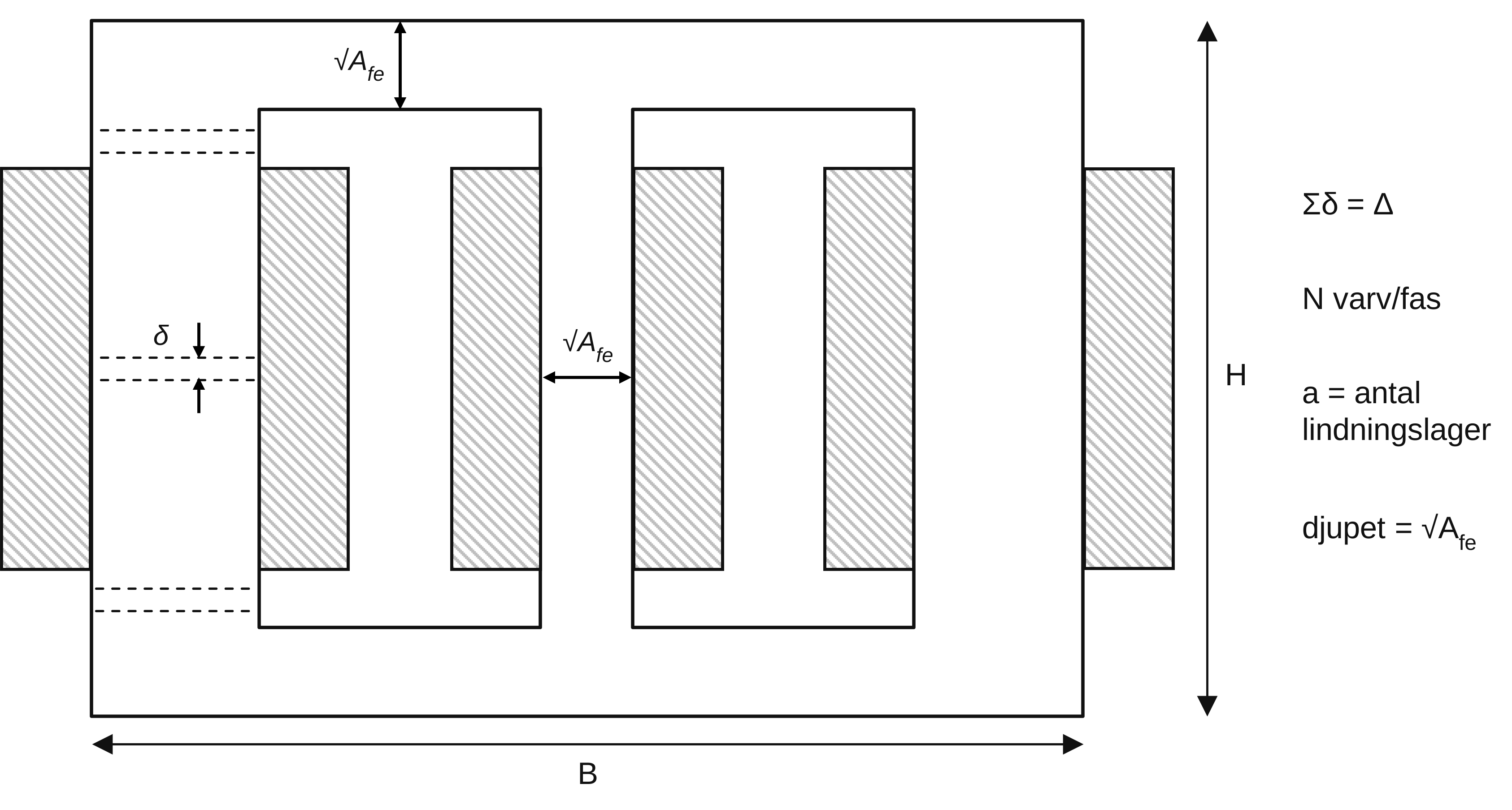
The air gaps are divided into several partial gaps to limit leakage flux.
B5.2 Calculation Procedure
The voltage induced in the winding is
\[e=\frac{d\Psi}{dt} \quad\Longrightarrow\quad \bar E=j\omega\Psi, \qquad E=\omega\Psi.\]Furthermore,
\[\Psi=N\Phi=NB A_{\mathrm{fe}},\]and therefore
\[E=2\pi B A_{\mathrm{fe}}Nf.\]With $\hat B$ expressed in gauss and $A_{\mathrm{fe}}$ in $\mathrm{cm}^2$ gives
\[E = \sqrt{2}\,\pi\,10^{-8} \hat B A_{\mathrm{fe}}Nf \qquad (\mathrm{cgs}).\]In addition,
\[\oint H\,ds=NI,\]which, for the iron path and the air gap, is written
\[H_{\Delta}\Delta+H_j\ell=NI.\]With
\[H_{\Delta}=\frac{B}{\mu_0}, \qquad H_j=\frac{B}{\mu\mu_0},\]gives
\[\frac{B}{\mu_0}\Delta + \frac{B}{\mu\mu_0}\ell = NI.\]The air-gap reluctance is assumed to dominate, so that
\[I=\frac{1}{\mu_0}\frac{B\Delta}{N}.\]For the rms value of the current and the peak value $\hat B$, this becomes
\[I = \frac{1}{\mu_0} \frac{\hat B\Delta}{N\sqrt{2}} 10^{-6} \qquad (\mathrm{cgs}),\]and hence
\[\Delta = \frac{\mu_0\sqrt{2}\,10^6IN}{\hat B} = \frac{0.4\pi\sqrt{2}\,IN}{\hat B} \qquad (\mathrm{cgs}).\]The reactance is
\[X = \frac{E}{I} = \frac{\sqrt{2}\,\pi\,10^{-8}\hat B f}{I} \,N A_{\mathrm{fe}} \qquad (\mathrm{cgs}).\]If the inductor is designed for the MBK 280 S-6 machine, the following is required:
\[I=160\ \mathrm{A}.\]Substitution of this together with the maximum current-density and flux-density values gives
\[\hat B=12\,000\ \mathrm{gauss}, \qquad S_{\max}=1.9\ \mathrm{A/mm^2}.\]Thus,
\[X = 1.66\cdot10^{-4} N A_{\mathrm{fe}} \qquad (\mathrm{cgs}),\]and
\[\Delta = 2.37\cdot10^{-2}N.\]Here $X$ is expressed in ohms and $\Delta$ in cm when $A_{\mathrm{fe}}$ is expressed in $\mathrm{cm}^2$.
B5.3 Copper Weights
At the current density
\[S=1.9\ \mathrm{A/mm^2}\]the required copper area is
\[A_{\mathrm{cu}} = \frac{160}{1.9} \approx 84\ \mathrm{mm^2} = 6\cdot14\ \mathrm{mm^2}.\]The conductor is therefore assumed to have the dimensions
\[b=6\ \mathrm{mm}, \qquad h=14\ \mathrm{mm},\]and the copper density is taken as
\[\rho_{\mathrm{cu}}=7900\ \mathrm{kg/m^3}.\]The copper weight for the three phases is
\[m_{\mathrm{cu}} = 3N A_{\mathrm{cu}}\ell\rho_{\mathrm{cu}},\]where the winding length per turn is approximated as
\[\ell = 4\left(\sqrt{A_{\mathrm{fe}}}+0.3a\right).\]Substitution gives
\[\begin{aligned} m_{\mathrm{cu}} &= 3A_{\mathrm{cu}}\rho_{\mathrm{cu}} \,4\left(\sqrt{A_{\mathrm{fe}}}+0.3a\right)N \\ &= 0.0796 \left(\sqrt{A_{\mathrm{fe}}}+0.3a\right)N, \end{aligned}\]where $A_{\mathrm{fe}}$ is expressed in $\mathrm{cm}^2$ and the mass in kg.
B5.4 Iron Weights
Limbs
The iron weight of the three limbs is written
\[m_{\mathrm{feb}} = 3A_{\mathrm{fe}}H\rho_{\mathrm{fe}},\]where
\[H=\frac{Nh}{a}+0.04.\]With $\rho = 2.2 \cdot 10^{-8}\ \Omega\mathrm{m}$ and $h=14\ \mathrm{mm}$ gives
\[\begin{aligned} m_{\mathrm{feb}} &= 3\rho_{\mathrm{fe}} \left(\frac{Nh}{a}+0.04\right) A_{\mathrm{fe}} \\ &= 3\cdot7900\cdot10^{-6} \left(\frac{Nh}{a}+4\right) A_{\mathrm{fe}} \\ &= 0.0237 \left(1.4\frac{N}{a}+4\right) A_{\mathrm{fe}}. \end{aligned}\]Here $A_{\mathrm{fe}}$ is expressed in $\mathrm{cm}^2$ and the mass in kg.
Yokes
The iron weight of the two yokes is written
\[m_{\mathrm{feo}} = 2A_{\mathrm{fe}}B\rho_{\mathrm{fe}},\]where the width of the core is approximated as
\[B = 3\sqrt{A_{\mathrm{fe}}} + 4\cdot1.2\,a b + 2\cdot0.03.\]This gives
\[\begin{aligned} m_{\mathrm{feo}} &= 2\rho_{\mathrm{fe}} \left( 3\sqrt{A_{\mathrm{fe}}} + 4.8ab + 0.06 \right) A_{\mathrm{fe}} \\ &= 2\cdot7900\cdot10^{-6} \left( 3\sqrt{A_{\mathrm{fe}}} + 2.88a + 6 \right) A_{\mathrm{fe}} \\ &= 0.0158 \left( 3\sqrt{A_{\mathrm{fe}}} + 2.88a + 6 \right) A_{\mathrm{fe}}. \end{aligned}\]Here too, $A_{\mathrm{fe}}$ is expressed in $\mathrm{cm}^2$ and the mass in kg.
B5.5 Summary
The expressions used can be summarized as
\[X = \frac{\sqrt{2}\,\pi\,10^{-8}\hat B f}{I} \,N A_{\mathrm{fe}} = 1.66\cdot10^{-4} N A_{\mathrm{fe}} \quad [\Omega],\] \[\Delta = \frac{\mu_0\sqrt{2}\,10^6 I}{\hat B}N = 2.37\cdot10^{-2}N \quad [\mathrm{cm}],\] \[m_{\mathrm{cu}} = 0.0897 \left( \sqrt{A_{\mathrm{fe}}}+0.3a \right)N,\] \[m_{\mathrm{feb}} = 0.0237 \left( 1.4\frac{N}{a}+4 \right) A_{\mathrm{fe}},\]and
\[m_{\mathrm{feo}} = 0.0158 \left( 3\sqrt{A_{\mathrm{fe}}}+2.88a+6 \right) A_{\mathrm{fe}}.\]If calculations are performed for three different inductors—0.5, 1.0, and 2.0 mH— the three diagrams in Figures 1–3 are obtained. In these, the inductor weight was calculated with limb area and the number of winding layers as free variables.
Appendix B6. Type Data
B6.1 Inverter
The DC-link voltage is
\[U_d = 488\ \mathrm{V}.\]| Operating mode | Fundamental-frequency range | $p$ | $m$ | $J’$ | $\alpha$ |
|---|---|---|---|---|---|
| A | 0.00–4.51 | 17 | 0 | 3 | 8.7, 24.4, 28.8 |
| B | 3.93–5.89 | 13 | 0 | 2 | 16.2, 22.1 |
| C | 5.47–10.95 | 7 | 0 | 1 | 12 |
| D | 9.60–12.77 | 6 | 0 | 1 | 12 |
| E | 11.52–15.32 | 5 | 0 | 1 | 12 |
| F | 14.02–17.88 | 5 | 0 | ||
| G | 17.53–22.35 | 4 | 0 | ||
| H | 21.28–25.92 | 3 | 0 | ||
| I | 25.54–41.44 | 2 | 0 | ||
| K | 39.06–50.00 | 1 | 0 | ||
| L | 50.00– | — | 0 |
B6.2 Motor
The motor is an MBK 280 S-6 with forced cooling.
Electrical Data
| Quantity | Value |
|---|---|
| Rated voltage, $U_n$ | $380\ \mathrm{V}$ |
| Rated current, $I_n$ | $150\ \mathrm{A}$ |
| Rated torque, $M_n$ | $740\ \mathrm{Nm}$ |
| Rated speed, $n_n$ | $970\ \mathrm{rpm}$ |
| Rated output power, $P_{2n}$ | $75\ \mathrm{kW}$ |
| Stator resistance | $0.062\ \Omega/\text{phase}$ |
| Stator reactance | $0.379\ \Omega/\text{phase}$ |
| Magnetizing reactance | $13.89\ \Omega/\text{phase}$ |
| Rotor reactance | $0.539\ \Omega/\text{phase}$ |
| Rotor resistance | $0.058\ \Omega/\text{phase}$ |
Mechanical Data
Stator:
| Quantity | Value |
|---|---|
| Stator diameter | 450 mm |
| Air-gap diameter | 335 mm |
| Lamination-stack length | $205\ \mathrm{mm}$ |
| Tooth height | $43.5\ \mathrm{mm}$ |
| Slot width | $10.1\ \mathrm{mm}$ |
| Tooth width | 8.2 mm |
| Winding weight | 47.2 kg |
| Number of slots | 54 |
Rotor:
| Quantity | Value |
|---|---|
| Tooth height | $29.5\ \mathrm{mm}$ |
| Slot width | $4.25\ \mathrm{mm}$ |
| Tooth width | 11.6 mm |
| Winding weight | 29.4 kg |
| Number of slots | 66 |
The total motor weight is
\[m_{\mathrm{tot}} = 480\ \mathrm{kg}.\]B6.3 Slot Data
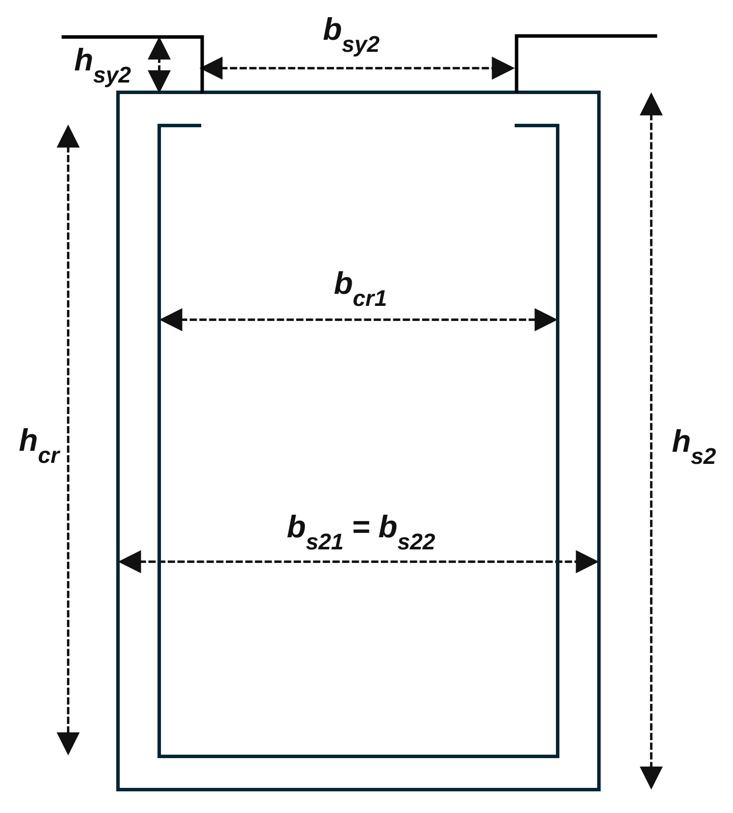
The handwritten annotations to the figure state:
SPTR: slot type according to theRESISTprogram $\rho_2$: conductor resistivity- $R_{\mathrm{rat}}$: ratio of the slot mean diameter to the rotor mean diameter
| Parameter | Value |
|---|---|
SPTR |
2 |
| $b_{s21}$ | $3.95\ \mathrm{mm}$ |
| $b_{s22}$ | $3.95\ \mathrm{mm}$ |
| $h_{s2}$ | $29.2\ \mathrm{mm}$ |
| $b_{sy2}$ | $2.0\ \mathrm{mm}$ |
| $h_{sy2}$ | $1.0\ \mathrm{mm}$ |
| $b_{cr1}$ | $3.75\ \mathrm{mm}$ |
| $h_{cr}$ | $28\ \mathrm{mm}$ |
| $\rho_2$ | $0.0425\ \Omega/\mathrm{m}$ |
| $R_{\mathrm{rat}}$ | $0.65$ |
Appendix B7. List of Variables
| Symbol | Meaning |
|---|---|
| $a$ | number of phases |
| $B$ | flux density |
| $B_{\max}$ | maximum flux density |
| $d$ | penetration depth |
| $E$ | flux voltage |
| $e$ | instantaneous value of the flux voltage |
| $f$ | frequency |
| $I_1$ | stator current |
| $I_2$ | rotor current |
| $I_{11}$ | fundamental stator current |
| $I_{1ö}$ | harmonic stator current |
| $I_{2ö}$ | harmonic rotor current |
| $k_h$ | proportionality factor |
| $k_v$ | proportionality factor |
| $L$ | inductor inductance |
| $L_1$ | stator inductance |
| $L_2$ | rotor inductance |
| $L_m$ | magnetizing inductance |
| $M$ | torque |
| $m$ | pulse ratio |
| $M_n$ | rated torque |
| $M_p$ | pulsating torque |
| $M(\theta)$ | modulation signal |
| $M_i$ | Fourier coefficient of $M(\theta)$ |
| $N$ | number of modulation pulses |
| $N_1$ | primary winding turns |
| $N_2$ | secondary winding turns |
| $P_{cu}$ | copper losses |
| $P_{cuö}$ | harmonic copper losses |
| $P_{fe}$ | iron losses |
| $P_{feö}$ | harmonic iron losses |
| $P_h$ | hysteresis losses |
| $P_v$ | eddy-current losses |
| $R$ | inductor resistance |
| $R_1$ | stator resistance |
| $R_2$ | rotor resistance |
| $R(\varphi)$ | reference signal |
| $R_n$ | Fourier coefficient of $R(\varphi)$ |
| $s$ | slip |
| $U$ | motor-terminal voltage |
| $U_1$ | fundamental of $U$ |
| $U_ö$ | harmonics of $U$ |
| $V$ | inverter-terminal voltage |
| $V_1$ | fundamental of $V$ |
| $V_{ö}$ | harmonics of $V$ |
| $Z_2$ | $jX_m \parallel \left(\dfrac{R_2}{s}+jX_2\right)$ |
| $\alpha_i$ | notch angles |
| $\beta$ | angle between the q-axis and the rotor r-axis |
| $\gamma$ | $U$, $I$, or $\Psi$ |
| $\theta$ | angle between the q-axis and the stator r-axis |
| $\theta_0$ | phase shift |
| $\theta_r$ | $\theta-\beta$ |
| $\lambda$ | exponent constant for hysteresis losses |
| $\xi$ | derating |
| $\sigma$ | conductivity |
| $\Phi$ | flux |
| $\varphi$ | angle, $\varphi=\omega t$ |
| $\Psi$ | flux linkage |
| $\omega$ | synchronous angular velocity |
| $\omega_e$ | electrical angular velocity |
| $\omega_r$ | rotor angular velocity |